Design and Analysis of Algorithms

Unit-I 

Asymptotic Notations and Introduction to Algorithms

An algorithm, named after the ninth century scholar Abu Jafar Muhammad Ibn Musu Al-Khowarizmi, is defined as follows: Roughly speaking:

• An algorithm is a set of rules for carrying out calculation either by hand or on a machine.
• An algorithm is a finite step-by-step procedure to achieve a required result.
• An algorithm is a sequence of computational steps that transform the input into the output.
• An algorithm is a sequence of operations performed on data that have to be organized in data structures.
• An algorithm is an abstraction of a program to be executed on a physical machine (model of Computation)

[http://www.personal.kent.edu/~rmuhamma/Algorithms/MyAlgorithms/intro.htm]

An algorithm is a recipe or a systematic method containing a sequence of instructions to solve a computational problem. It takes some inputs, performs a well de ned sequence of steps, and produces some output. Once we design an algorithm, we need to know how well it performs on any input. In particular we would like to know whether there are better algorithms for the problem. An answer to this rst demands a way to analyze an algorithm in a machine-independent way. Algorithm design and analysis form a central theme in computer science.

[http://www.imsc.res.in/~vraman/pub/intro_notes.pdf]

Algorithmic is a branch of computer science that consists of designing and analyzing computer algorithms

1. The “design” pertain to

i. The description of algorithm at an abstract level by means of a pseudo language, and
ii. Proof of correctness that is, the algorithm solves the given problem in all cases.

2. The “analysis” deals with performance evaluation (complexity analysis).

We start with defining the model of computation, which is usually the Random Access Machine (RAM) model, but other models of computations can be use such as PRAM. Once the model of computation has been defined, an algorithm can be describe using a simple language (or pseudo language) whose syntax is close to programming language such as C or java.

Algorithm is a step-by-step procedure, which defines a set of instructions to be executed in a certain order to get the desired output. Algorithms are generally created independent of underlying languages, i.e. an algorithm can be implemented in more than one programming language.

From the data structure point of view, following are some important categories of algorithms −

• Search − Algorithm to search an item in a data structure.
• Sort − Algorithm to sort items in a certain order.
• Insert − Algorithm to insert item in a data structure.
• Update − Algorithm to update an existing item in a data structure.
• Delete − Algorithm to delete an existing item from a data structure.

Characteristics of an Algorithm

Not all procedures can be called an algorithm. An algorithm should have the following characteristics −

• Unambiguous − Algorithm should be clear and unambiguous. Each of its steps (or phases), and their inputs/outputs should be clear and must lead to only one meaning.
• Input − An algorithm should have 0 or more well-defined inputs.
• Output − An algorithm should have 1 or more well-defined outputs, and should match the desired output.
• Finiteness − Algorithms must terminate after a finite number of steps.
• Feasibility − Should be feasible with the available resources.
• Independent − An algorithm should have step-by-step directions, which should be independent of any programming code.

How to Write an Algorithm?

There are no well-defined standards for writing algorithms. Rather, it is problem and resource dependent. Algorithms are never written to support a particular programming code.

As we know that all programming languages share basic code constructs like loops (do, for, while), flow-control (if-else), etc. These common constructs can be used to write an algorithm.

We write algorithms in a step-by-step manner, but it is not always the case. Algorithm writing is a process and is executed after the problem domain is well-defined. That is, we should know the problem domain, for which we are designing a solution.

Example

Let's try to learn algorithm-writing by using an example.

Problem − Design an algorithm to add two numbers and display the result.

step 1 − START
step 2 − declare three integers a, b & c
step 3 − define values of a & b
step 4 − add values of a & b
step 5 − store output of step 4 to c
step 6 − print c
step 7 − STOP

Algorithms tell the programmers how to code the program. Alternatively, the algorithm can be written as −

step 1 − START ADD
step 2 − get values of a & b
step 3 − c ← a + b
step 4 − display c
step 5 − STOP

In design and analysis of algorithms, usually the second method is used to describe an algorithm. It makes it easy for the analyst to analyze the algorithm ignoring all unwanted definitions. He can observe what operations are being used and how the process is flowing.

Writing step numbers, is optional.

We design an algorithm to get a solution of a given problem. A problem can be solved in more than one ways.

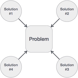
Hence, many solution algorithms can be derived for a given problem. The next step is to analyze those proposed solution algorithms and implement the best suitable solution.

Algorithm Analysis

Efficiency of an algorithm can be analyzed at two different stages, before implementation and after implementation. They are the following −

• A Priori Analysis − This is a theoretical analysis of an algorithm. Efficiency of an algorithm is measured by assuming that all other factors, for example, processor speed, are constant and have no effect on the implementation.
• A Posterior Analysis − This is an empirical analysis of an algorithm. The selected algorithm is implemented using programming language. This is then executed on target computer machine. In this analysis, actual statistics like running time and space required, are collected.

We shall learn about a priori algorithm analysis. Algorithm analysis deals with the execution or running time of various operations involved. The running time of an operation can be defined as the number of computer instructions executed per operation.

Algorithm Complexity

Suppose X is an algorithm and n is the size of input data, the time and space used by the algorithm X are the two main factors, which decide the efficiency of X.

• Time Factor − Time is measured by counting the number of key operations such as comparisons in the sorting algorithm.
• Space Factor − Space is measured by counting the maximum memory space required by the algorithm.

The complexity of an algorithm f(n) gives the running time and/or the storage space required by the algorithm in terms of n as the size of input data.

Space Complexity

Space complexity of an algorithm represents the amount of memory space required by the algorithm in its life cycle. The space required by an algorithm is equal to the sum of the following two components −

• A fixed part that is a space required to store certain data and variables, that are independent of the size of the problem. For example, simple variables and constants used, program size, etc.
• A variable part is a space required by variables, whose size depends on the size of the problem. For example, dynamic memory allocation, recursion stack space, etc.

Space complexity S(P) of any algorithm P is S(P) = C + SP(I), where C is the fixed part and S(I) is the variable part of the algorithm, which depends on instance characteristic I. Following is a simple example that tries to explain the concept −

Algorithm: SUM(A, B)
Step 1 -  START
Step 2 -  C ← A + B + 10
Step 3 -  Stop

Here we have three variables A, B, and C and one constant. Hence S(P) = 1 + 3. Now, space depends on data types of given variables and constant types and it will be multiplied accordingly.

Time Complexity

Time complexity of an algorithm represents the amount of time required by the algorithm to run to completion. Time requirements can be defined as a numerical function T(n), where T(n) can be measured as the number of steps, provided each step consumes constant time.

For example, addition of two n-bit integers takes n steps. Consequently, the total computational time is T(n) = c ∗ n, where c is the time taken for the addition of two bits. Here, we observe that T(n) grows linearly as the input size increases.

Asymptotic Notation

Asymptotic analysis of an algorithm refers to defining the mathematical boundation/framing of its run-time performance. Using asymptotic analysis, we can very well conclude the best case, average case, and worst case scenario of an algorithm.

Asymptotic analysis is input bound i.e., if there's no input to the algorithm, it is concluded to work in a constant time. Other than the "input" all other factors are considered constant.

Asymptotic analysis refers to computing the running time of any operation in mathematical units of computation. For example, the running time of one operation is computed as f(n) and may be for another operation it is computed as g(n²). This means the first operation running time will increase linearly with the increase in n and the running time of the second operation will increase exponentially when n increases. Similarly, the running time of both operations will be nearly the same if n is significantly small.

Usually, the time required by an algorithm falls under three types −

• Best Case − Minimum time required for program execution.
• Average Case − Average time required for program execution.
• Worst Case − Maximum time required for program execution.

Asymptotic Notations

Following are the commonly used asymptotic notations to calculate the running time complexity of an algorithm.

• Ο Notation
• Ω Notation
• θ Notation

Big Oh Notation, Ο

The notation Ο(n) is the formal way to express the upper bound of an algorithm's running time. It measures the worst case time complexity or the longest amount of time an algorithm can possibly take to complete.

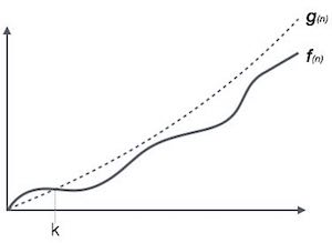
For example, for a function f(n)

Ο(f(n)) = { g(n) : there exists c > 0 and n0 such that f(n) ≤ c.g(n) for all n > n0. }

Omega Notation, Ω

The notation Ω(n) is the formal way to express the lower bound of an algorithm's running time. It measures the best case time complexity or the best amount of time an algorithm can possibly take to complete.

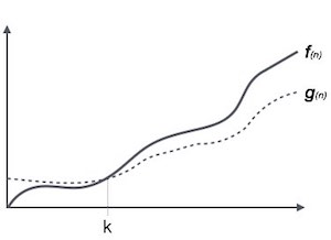
For example, for a function f(n)

Ω(f(n)) ≥ { g(n) : there exists c > 0 and n0 such that g(n) ≤ c.f(n) for all n > n0. }

Theta Notation, θ

The notation θ(n) is the formal way to express both the lower bound and the upper bound of an algorithm's running time. It is represented as follows −

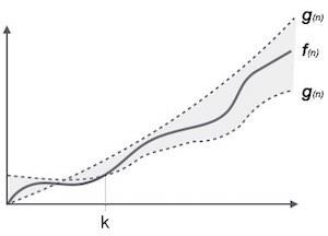
θ(f(n)) = { g(n) if and only if g(n) =  Ο(f(n)) and g(n) = Ω(f(n)) for all n > n0. }

Common Asymptotic Notations

Following is a list of some common asymptotic notations −

constant	−	Ο(1)
logarithmic	−	Ο(log n)
linear	−	Ο(n)
n log n	−	Ο(n log n)
quadratic	−	Ο(n2)
cubic	−	Ο(n3)
polynomial	−	nΟ(1)
exponential	−	2Ο(n)

[https://www.tutorialspoint.com/data_structures_algorithms/asymptotic_analysis.htm]

Analysis of algorithms 

The theoretical study of computer-program performance and resource usage.
What’s more important than performance?
• modularity
• correctness
• maintainability
• functionality
• robustness
• user-friendliness
• programmer time
• simplicity
• extensibility
• reliability

Why study algorithms and performance? 

• Algorithms help us to understand scalability.
• Performance often draws the line between what is feasible and what is impossible.
• Algorithmic mathematics provides a language for talking about program behavior.
• The lessons of program performance generalize to other computing resources.

Running time 

• The running time depends on the input: an already sorted sequence is easier to sort.
• Parameterize the running time by the size of the input, since short sequences are easier to sort than long ones.
• Generally, we seek upper bounds on the running time, because everybody likes a guarantee.
Kinds of analyses
Worst-case: (usually)
• T(n) = maximum time of algorithm on any input of size n.
Average-case: (sometimes)
• T(n) = expected time of algorithm on any input of size n.
Best-case: (bogus)
• Cheat with a slow algorithm that works fast on some input.
[http://www.facweb.iitkgp.ernet.in/~sourav/Lecture-01.pdf]

Classification of Algorithms

• Classification by purpose

• By implementation

• By design paradigm

• By complexity

Classification by purpose
Classification by implementation

• Recursive or iterative

• A recursive algorithm is one that calls itself repeatedly until a certain condition matches. It is a method common to functional programming. 

• Iterative algorithms use repetitive constructs like loops.

• Some problems are better suited for one implementation or the other. For example, the towers of hanoi problem is well understood in recursive implementation. Every recursive version has an iterative equivalent iterative, and vice versa.

• Logical or procedural

• An algorithm may be viewed as controlled logical deduction. 

• A logic component expresses the axioms which may be used in the computation and a control component determines the way in which deduction is applied to the axioms. 

• This is the basis of the logic programming. In pure logic programming languages the control component is fixed and algorithms are specified by supplying only the logic component.

• Serial or parallel

• Algorithms are usually discussed with the assumption that computers execute one instruction of an algorithm at a time. This is a serial algorithm, as opposed to parallel algorithms, which take advantage of computer architectures to process several instructions at once. They divide the problem into sub-problems and pass them to several processors. Iterative algorithms are generally parallelizable. Sorting algorithms can be parallelized efficiently.

• Deterministic or non-deterministic

• Deterministic algorithms solve the problem with a predefined process whereas non-deterministic algorithm must perform guesses of best solution at each step through the use of heuristics.

Classification by design paradigm

• Divide and conquer

• A divide and conquer algorithm repeatedly reduces an instance of a problem to one or more smaller instances of the same problem (usually recursively), until the instances are small enough to solve easily. One such example of divide and conquer is merge sorting. Sorting can be done on each segment of data after dividing data into segments and sorting of entire data can be obtained in conquer phase by merging them. 

• The binary search algorithm is an example of a variant of divide and conquer called decrease and conquer algorithm, that solves an identical subproblem and uses the solution of this subproblem to solve the bigger problem. 

• 
  

• Dynamic programming

• The shortest path in a weighted graph can be found by using the shortest path to the goal from all adjacent vertices. 

• When the optimal solution to a problem can be constructed from optimal solutions to subproblems, using dynamic programming avoids recomputing solutions that have already been computed. 

• - The main difference with the "divide and conquer" approach is, subproblems are independent in divide and conquer, where as the overlap of subproblems occur in dynamic programming. 

• - Dynamic programming and memoization go together. The difference with straightforward recursion is in caching or memoization of recursive calls. Where subproblems are independent, this is useless. By using memoization or maintaining a table of subproblems already solved, dynamic programming reduces the exponential nature of many problems to polynomial complexity.

•  

• The greedy method

• A greedy algorithm is similar to a dynamic programming algorithm, but the difference is that solutions to the subproblems do not have to be known at each stage. Instead a "greedy" choice can be made of what looks the best solution for the moment. 

• The most popular greedy algorithm is finding the minimal spanning tree as given by Kruskal.

•  

• Linear programming

• The problem is expressed as a set of linear inequalities and then an attempt is made to maximize or minimize the inputs. This can solve many problems such as the maximum flow for directed graphs, notably by using the simplex algorithm. 

• A complex variant of linear programming is called integer programming, where the solution space is restricted to all integers.

•  

• Reduction also called transform and conquer

• Solve a problem by transforming it into another problem. A simple example: finding the median in an unsorted list is first translating this problem into sorting problem and finding the middle element in sorted list. The main goal of reduction is finding the simplest transformation possible.

•  

• Using graphs

• Many problems, such as playing chess, can be modeled as problems on graphs. A graph exploration algorithms are used. 

• This category also includes the search algorithms and backtracking.

•  

• The probabilistic and heuristic paradigm 

• 
  

1. Probabilistic 

1. Those that make some choices randomly.

1. Genetic 

1. Attempt to find solutions to problems by mimicking biological evolutionary processes, with a cycle of random mutations yielding successive generations of "solutions". Thus, they emulate reproduction and "survival of the fittest".

1. Heuristic 

1. Whose general purpose is not to find an optimal solution, but an approximate solution where the time or resources to find a perfect solution are not practical.

Classification by complexity

On Scriptol.org, algorithms are classified by purpose, but there are other ways to classify them.

Each algorithm has a goal, for example, the purpose of the Quick Sort algorithm is to sort data in ascending or descending order. But the number of goals is infinite, and we have to group them by kind of purposes.

An algorithm may be implemeted according to different basical principles.

A design paradigm is a domain in research or class of problems that requires a dedicated kind of algorithm:

Some algorithms complete in linear time, and some complete in exponential amount of time, and some never complete.

[http://www.scriptol.com/programming/algorithms-classification.php]

BASIC DIFFERENCES BETWEEN SPACE COMPLEXITY AND TIME COMPLEXITY

SPACE COMPLEXITY:

The space complexity of an algorithm is the amount of memory it requires to run to completion.

the space needed by a program contains the following components:

1)  Instruction space:

-stores the executable version of programs and is generally fixed.

2) Data space:

It contains:

a)  Space required by constants and simple variables.Its space is fixed.

b)  Space needed by fixed size stucture variables such as array and structures.

c)  dynamically allocated space.This space is usually variable.

3) enviorntal stack:

-Needed to stores information required to reinvoke suspended processes or functions.

the following data is saved on the stack

- return address.

-value of all local variables

-value of all formal parameters in the function..

TIME COMPLEXITY:

The time complexity of an algorithm is the amount of time it needs to run to completion. namely space

To measure the time complexity we can count all operations performed in an algorithm and if we know the time taken for each operation then we can easily compute the total time taken by the algorithm.This time varies from system to system.

Our intention is to estimate execution time of an algorithm irrespective of the computer on which it will be used. Hence identify the key operation and count such operation performed till the program completes its execution.

The time complexity can be expressd as a function of a key operation performed.

The space and time complexity is usually expressed in the form of function f(n),where n is the input size for a given instance of a problem being solved.

f(n) helps us to predict the rate of growthof complexity that will increase as size of input to the problem increases.

f(1) also helps us to predict complexity of two or more algorithms in order ro find which is more efficient.

[https://www.boddunan.com/articles/education/22-computer-science/18117-differences-between-space-complexity-and-time-complexity-space-complexity.html]

Recurrence Relations

Read PDF file whose link is :

[https://www.cs.duke.edu/~reif/courses/alglectures/skiena.lectures/lecture3.pdf]

Sorting Techniques

Sorting refers to arranging data in a particular format. Sorting algorithm specifies the way to arrange data in a particular order. Most common orders are in numerical or lexicographical order.

The importance of sorting lies in the fact that data searching can be optimized to a very high level, if data is stored in a sorted manner. Sorting is also used to represent data in more readable formats. Following are some of the examples of sorting in real-life scenarios −

• Telephone Directory − The telephone directory stores the telephone numbers of people sorted by their names, so that the names can be searched easily.
• Dictionary − The dictionary stores words in an alphabetical order so that searching of any word becomes easy.

In-place Sorting and Not-in-place Sorting

Sorting algorithms may require some extra space for comparison and temporary storage of few data elements. These algorithms do not require any extra space and sorting is said to happen in-place, or for example, within the array itself. This is called in-place sorting. Bubble sort is an example of in-place sorting.

However, in some sorting algorithms, the program requires space which is more than or equal to the elements being sorted. Sorting which uses equal or more space is called not-in-place sorting. Merge-sort is an example of not-in-place sorting.

Stable and Not Stable Sorting

If a sorting algorithm, after sorting the contents, does not change the sequence of similar content in which they appear, it is called stable sorting.

If a sorting algorithm, after sorting the contents, changes the sequence of similar content in which they appear, it is called unstable sorting.

Stability of an algorithm matters when we wish to maintain the sequence of original elements, like in a tuple for example.

Adaptive and Non-Adaptive Sorting Algorithm

A sorting algorithm is said to be adaptive, if it takes advantage of already 'sorted' elements in the list that is to be sorted. That is, while sorting if the source list has some element already sorted, adaptive algorithms will take this into account and will try not to re-order them.

A non-adaptive algorithm is one which does not take into account the elements which are already sorted. They try to force every single element to be re-ordered to confirm their sortedness.

Important Terms

Some terms are generally coined while discussing sorting techniques, here is a brief introduction to them −

Increasing Order

A sequence of values is said to be in increasing order, if the successive element is greater than the previous one. For example, 1, 3, 4, 6, 8, 9 are in increasing order, as every next element is greater than the previous element.

Decreasing Order

A sequence of values is said to be in decreasing order, if the successive element is less than the current one. For example, 9, 8, 6, 4, 3, 1 are in decreasing order, as every next element is less than the previous element.

Non-Increasing Order

A sequence of values is said to be in non-increasing order, if the successive element is less than or equal to its previous element in the sequence. This order occurs when the sequence contains duplicate values. For example, 9, 8, 6, 3, 3, 1 are in non-increasing order, as every next element is less than or equal to (in case of 3) but not greater than any previous element.

Non-Decreasing Order

A sequence of values is said to be in non-decreasing order, if the successive element is greater than or equal to its previous element in the sequence. This order occurs when the sequence contains duplicate values. For example, 1, 3, 3, 6, 8, 9 are in non-decreasing order, as every next element is greater than or equal to (in case of 3) but not less than the previous one.

Bubble Sort Algorithm

Bubble sort is a simple sorting algorithm. This sorting algorithm is comparison-based algorithm in which each pair of adjacent elements is compared and the elements are swapped if they are not in order. This algorithm is not suitable for large data sets as its average and worst case complexity are of Ο(n²) where n is the number of items.

How Bubble Sort Works?

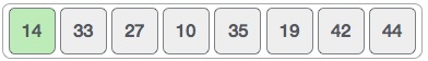
We take an unsorted array for our example. Bubble sort takes Ο(n²) time so we're keeping it short and precise.

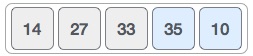
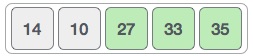
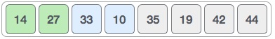
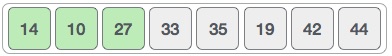
Bubble sort starts with very first two elements, comparing them to check which one is greater.

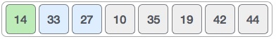
In this case, value 33 is greater than 14, so it is already in sorted locations. Next, we compare 33 with 27.

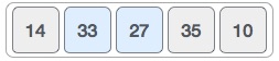
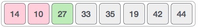
We find that 27 is smaller than 33 and these two values must be swapped.

The new array should look like this −

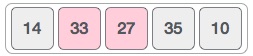
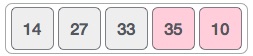
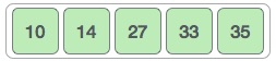
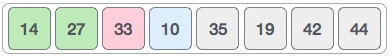
Next we compare 33 and 35. We find that both are in already sorted positions.

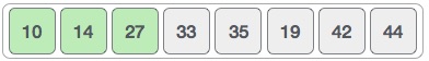
Then we move to the next two values, 35 and 10.

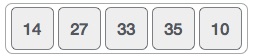
We know then that 10 is smaller 35. Hence they are not sorted.

We swap these values. We find that we have reached the end of the array. After one iteration, the array should look like this −

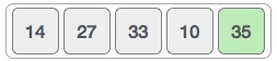
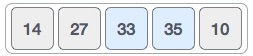
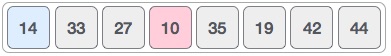
To be precise, we are now showing how an array should look like after each iteration. After the second iteration, it should look like this −

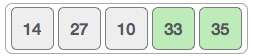
Notice that after each iteration, at least one value moves at the end.

And when there's no swap required, bubble sorts learns that an array is completely sorted.

Now we should look into some practical aspects of bubble sort.

Algorithm

We assume list is an array of n elements. We further assume that swap function swaps the values of the given array elements.

begin BubbleSort(list)

   for all elements of list
      if list[i] > list[i+1]
         swap(list[i], list[i+1])
      end if
   end for
   
   return list
   
end BubbleSort

Pseudocode

We observe in algorithm that Bubble Sort compares each pair of array element unless the whole array is completely sorted in an ascending order. This may cause a few complexity issues like what if the array needs no more swapping as all the elements are already ascending.

To ease-out the issue, we use one flag variable swapped which will help us see if any swap has happened or not. If no swap has occurred, i.e. the array requires no more processing to be sorted, it will come out of the loop.

Pseudocode of BubbleSort algorithm can be written as follows −

procedure bubbleSort( list : array of items )

   loop = list.count;
   
   for i = 0 to loop-1 do:
      swapped = false
  
      for j = 0 to loop-1 do:
      
         /* compare the adjacent elements */   
         if list[j] > list[j+1] then
            /* swap them */
            swap( list[j], list[j+1] )   
            swapped = true
         end if
         
      end for
      
      /*if no number was swapped that means 
      array is sorted now, break the loop.*/
      
      if(not swapped) then
         break
      end if
      
   end for
   
end procedure return list

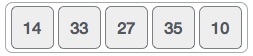
Insertion Sort

This is an in-place comparison-based sorting algorithm. Here, a sub-list is maintained which is always sorted. For example, the lower part of an array is maintained to be sorted. An element which is to be 'insert'ed in this sorted sub-list, has to find its appropriate place and then it has to be inserted there. Hence the name, insertion sort.

The array is searched sequentially and unsorted items are moved and inserted into the sorted sub-list (in the same array). This algorithm is not suitable for large data sets as its average and worst case complexity are of Ο(n²), where n is the number of items.

How Insertion Sort Works?

We take an unsorted array for our example.

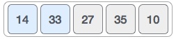
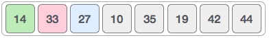
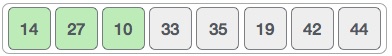
Insertion sort compares the first two elements.

It finds that both 14 and 33 are already in ascending order. For now, 14 is in sorted sub-list.

Insertion sort moves ahead and compares 33 with 27.

And finds that 33 is not in the correct position.

It swaps 33 with 27. It also checks with all the elements of sorted sub-list. Here we see that the sorted sub-list has only one element 14, and 27 is greater than 14. Hence, the sorted sub-list remains sorted after swapping.

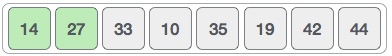
By now we have 14 and 27 in the sorted sub-list. Next, it compares 33 with 10.

These values are not in a sorted order.

So we swap them.

However, swapping makes 27 and 10 unsorted.

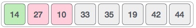
Hence, we swap them too.

Again we find 14 and 10 in an unsorted order.

We swap them again. By the end of third iteration, we have a sorted sub-list of 4 items.

This process goes on until all the unsorted values are covered in a sorted sub-list. Now we shall see some programming aspects of insertion sort.

Algorithm

Now we have a bigger picture of how this sorting technique works, so we can derive simple steps by which we can achieve insertion sort.

Step 1 − If it is the first element, it is already sorted. return 1;
Step 2 − Pick next element
Step 3 − Compare with all elements in the sorted sub-list
Step 4 − Shift all the elements in the sorted sub-list that is greater than the 
         value to be sorted
Step 5 − Insert the value
Step 6 − Repeat until list is sorted

Pseudocode

procedure insertionSort( A : array of items )
   int holePosition
   int valueToInsert
 
   for i = 1 to length(A) inclusive do:
 
      /* select value to be inserted */
      valueToInsert = A[i]
      holePosition = i
      
      /*locate hole position for the element to be inserted */
  
      while holePosition > 0 and A[holePosition-1] > valueToInsert do:
         A[holePosition] = A[holePosition-1]
         holePosition = holePosition -1
      end while
  
      /* insert the number at hole position */
      A[holePosition] = valueToInsert
      
   end for
 
end procedure

Selection Sort

Selection sort is a simple sorting algorithm. This sorting algorithm is an in-place comparison-based algorithm in which the list is divided into two parts, the sorted part at the left end and the unsorted part at the right end. Initially, the sorted part is empty and the unsorted part is the entire list.

The smallest element is selected from the unsorted array and swapped with the leftmost element, and that element becomes a part of the sorted array. This process continues moving unsorted array boundary by one element to the right.

This algorithm is not suitable for large data sets as its average and worst case complexities are of Ο(n²), where n is the number of items.

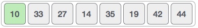
How Selection Sort Works?

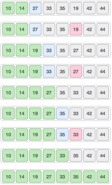
Consider the following depicted array as an example.

For the first position in the sorted list, the whole list is scanned sequentially. The first position where 14 is stored presently, we search the whole list and find that 10 is the lowest value.

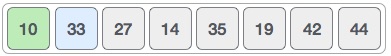
So we replace 14 with 10. After one iteration 10, which happens to be the minimum value in the list, appears in the first position of the sorted list.

For the second position, where 33 is residing, we start scanning the rest of the list in a linear manner.

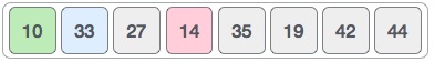
We find that 14 is the second lowest value in the list and it should appear at the second place. We swap these values.

After two iterations, two least values are positioned at the beginning in a sorted manner.

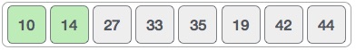
The same process is applied to the rest of the items in the array.

Following is a pictorial depiction of the entire sorting process −

Now, let us learn some programming aspects of selection sort.

Algorithm

Step 1 − Set MIN to location 0
Step 2 − Search the minimum element in the list
Step 3 − Swap with value at location MIN
Step 4 − Increment MIN to point to next element
Step 5 − Repeat until list is sorted

Pseudocode

procedure selection sort 
   list  : array of items
   n     : size of list

   for i = 1 to n - 1
   /* set current element as minimum*/
      min = i    
  
      /* check the element to be minimum */

      for j = i+1 to n 
         if list[j] < list[min] then
            min = j;
         end if
      end for

      /* swap the minimum element with the current element*/
      if indexMin != i  then
         swap list[min] and list[i]
      end if

   end for
 
end procedure

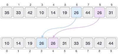
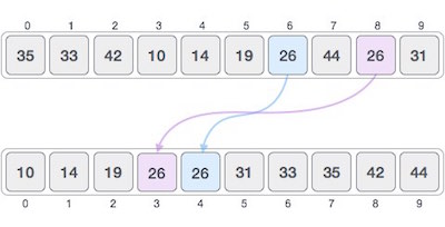
Merge Sort

Merge sort is a sorting technique based on divide and conquer technique. With worst-case time complexity being Ο(n log n), it is one of the most respected algorithms.

Merge sort first divides the array into equal halves and then combines them in a sorted manner.

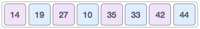
How Merge Sort Works?

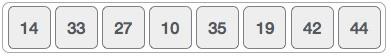
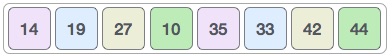
To understand merge sort, we take an unsorted array as the following −

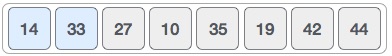
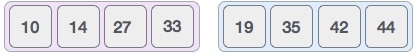
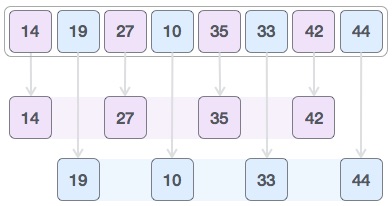
We know that merge sort first divides the whole array iteratively into equal halves unless the atomic values are achieved. We see here that an array of 8 items is divided into two arrays of size 4.

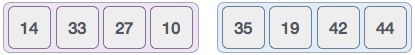
This does not change the sequence of appearance of items in the original. Now we divide these two arrays into halves.

We further divide these arrays and we achieve atomic value which can no more be divided.

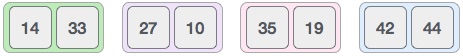
Now, we combine them in exactly the same manner as they were broken down. Please note the color codes given to these lists.

We first compare the element for each list and then combine them into another list in a sorted manner. We see that 14 and 33 are in sorted positions. We compare 27 and 10 and in the target list of 2 values we put 10 first, followed by 27. We change the order of 19 and 35 whereas 42 and 44 are placed sequentially.

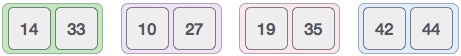
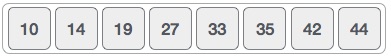
In the next iteration of the combining phase, we compare lists of two data values, and merge them into a list of found data values placing all in a sorted order.

After the final merging, the list should look like this −

Now we should learn some programming aspects of merge sorting.

Algorithm

Merge sort keeps on dividing the list into equal halves until it can no more be divided. By definition, if it is only one element in the list, it is sorted. Then, merge sort combines the smaller sorted lists keeping the new list sorted too.

Step 1 − if it is only one element in the list it is already sorted, return.
Step 2 − divide the list recursively into two halves until it can no more be divided.
Step 3 − merge the smaller lists into new list in sorted order.

Pseudocode

We shall now see the pseudocodes for merge sort functions. As our algorithms point out two main functions − divide & merge.

Merge sort works with recursion and we shall see our implementation in the same way.

procedure mergesort( var a as array )
   if ( n == 1 ) return a

   var l1 as array = a[0] ... a[n/2]
   var l2 as array = a[n/2+1] ... a[n]

   l1 = mergesort( l1 )
   l2 = mergesort( l2 )

   return merge( l1, l2 )
end procedure

procedure merge( var a as array, var b as array )

   var c as array

   while ( a and b have elements )
      if ( a[0] > b[0] )
         add b[0] to the end of c
         remove b[0] from b
      else
         add a[0] to the end of c
         remove a[0] from a
      end if
   end while
   
   while ( a has elements )
      add a[0] to the end of c
      remove a[0] from a
   end while
   
   while ( b has elements )
      add b[0] to the end of c
      remove b[0] from b
   end while
   
   return c
 
end procedure

Shell Sort

Shell sort is a highly efficient sorting algorithm and is based on insertion sort algorithm. This algorithm avoids large shifts as in case of insertion sort, if the smaller value is to the far right and has to be moved to the far left.

This algorithm uses insertion sort on a widely spread elements, first to sort them and then sorts the less widely spaced elements. This spacing is termed as interval. This interval is calculated based on Knuth's formula as −

Knuth's Formula

h = h * 3 + 1

where −
   h is interval with initial value 1

This algorithm is quite efficient for medium-sized data sets as its average and worst case complexity are of Ο(n), where n is the number of items.

How Shell Sort Works?

Let us consider the following example to have an idea of how shell sort works. We take the same array we have used in our previous examples. For our example and ease of understanding, we take the interval of 4. Make a virtual sub-list of all values located at the interval of 4 positions. Here these values are {35, 14}, {33, 19}, {42, 27} and {10, 14}

We compare values in each sub-list and swap them (if necessary) in the original array. After this step, the new array should look like this −

Then, we take interval of 2 and this gap generates two sub-lists - {14, 27, 35, 42}, {19, 10, 33, 44}

We compare and swap the values, if required, in the original array. After this step, the array should look like this −

Finally, we sort the rest of the array using interval of value 1. Shell sort uses insertion sort to sort the array.

Following is the step-by-step depiction −

We see that it required only four swaps to sort the rest of the array.

Algorithm

Following is the algorithm for shell sort.

Step 1 − Initialize the value of h
Step 2 − Divide the list into smaller sub-list of equal interval h
Step 3 − Sort these sub-lists using insertion sort
Step 3 − Repeat until complete list is sorted

Pseudocode

Following is the pseudocode for shell sort.

procedure shellSort()
   A : array of items 
 
   /* calculate interval*/
   while interval < A.length /3 do:
      interval = interval * 3 + 1     
   end while
   
   while interval > 0 do:

      for outer = interval; outer < A.length; outer ++ do:

      /* select value to be inserted */
      valueToInsert = A[outer]
      inner = outer;

         /*shift element towards right*/
         while inner > interval -1 && A[inner - interval] >= valueToInsert do:
            A[inner] = A[inner - interval]
            inner = inner - interval
         end while

      /* insert the number at hole position */
      A[inner] = valueToInsert

      end for

   /* calculate interval*/
   interval = (interval -1) /3;   

   end while
   
end procedure

Quick Sort

Quick sort is a highly efficient sorting algorithm and is based on partitioning of array of data into smaller arrays. A large array is partitioned into two arrays one of which holds values smaller than the specified value, say pivot, based on which the partition is made and another array holds values greater than the pivot value.

Quick sort partitions an array and then calls itself recursively twice to sort the two resulting subarrays. This algorithm is quite efficient for large-sized data sets as its average and worst case complexity are of Ο(nlogn), where n is the number of items.

Partition in Quick Sort

Following animated representation explains how to find the pivot value in an array.

The pivot value divides the list into two parts. And recursively, we find the pivot for each sub-lists until all lists contains only one element.

Quick Sort Pivot Algorithm

Based on our understanding of partitioning in quick sort, we will now try to write an algorithm for it, which is as follows.

Step 1 − Choose the highest index value has pivot
Step 2 − Take two variables to point left and right of the list excluding pivot
Step 3 − left points to the low index
Step 4 − right points to the high
Step 5 − while value at left is less than pivot move right
Step 6 − while value at right is greater than pivot move left
Step 7 − if both step 5 and step 6 does not match swap left and right
Step 8 − if left ≥ right, the point where they met is new pivot

Quick Sort Pivot Pseudocode

The pseudocode for the above algorithm can be derived as −

function partitionFunc(left, right, pivot)
   leftPointer = left -1
   rightPointer = right

   while True do
      while A[++leftPointer] < pivot do
         //do-nothing            
      end while
  
      while rightPointer > 0 && A[--rightPointer] > pivot do
         //do-nothing         
      end while
  
      if leftPointer >= rightPointer
         break
      else                
         swap leftPointer,rightPointer
      end if
  
   end while 
 
   swap leftPointer,right
   return leftPointer
 
end function

Quick Sort Algorithm

Using pivot algorithm recursively, we end up with smaller possible partitions. Each partition is then processed for quick sort. We define recursive algorithm for quicksort as follows −

Step 1 − Make the right-most index value pivot
Step 2 − partition the array using pivot value
Step 3 − quicksort left partition recursively
Step 4 − quicksort right partition recursively

Quick Sort Pseudocode

To get more into it, let see the pseudocode for quick sort algorithm −

procedure quickSort(left, right)

   if right-left <= 0
      return
   else     
      pivot = A[right]
      partition = partitionFunc(left, right, pivot)
      quickSort(left,partition-1)
      quickSort(partition+1,right)    
   end if  
   
end procedure

Insertion Sort Program in C

Implementation in C

#include <stdio.h>
#include <stdbool.h>
#define MAX 7

int intArray[MAX] = {4,6,3,2,1,9,7};

void printline(int count) {
   int i;
 
   for(i = 0;i <count-1;i++) {
      printf("=");
   }
 
   printf("=\n");
}

void display() {
   int i;
   printf("[");
 
   // navigate through all items 
   for(i = 0;i<MAX;i++) {
      printf("%d ",intArray[i]);
   }
 
   printf("]\n");
}

void insertionSort() {

   int valueToInsert;
   int holePosition;
   int i;
  
   // loop through all numbers 
   for(i = 1; i < MAX; i++) { 
 
      // select a value to be inserted. 
      valueToInsert = intArray[i];
  
      // select the hole position where number is to be inserted 
      holePosition = i;
  
      // check if previous no. is larger than value to be inserted 
      while (holePosition > 0 && intArray[holePosition-1] > valueToInsert) {
         intArray[holePosition] = intArray[holePosition-1];
         holePosition--;
         printf(" item moved : %d\n" , intArray[holePosition]);
      }

      if(holePosition != i) {
         printf(" item inserted : %d, at position : %d\n" , valueToInsert,holePosition);
         // insert the number at hole position 
         intArray[holePosition] = valueToInsert;
      }

      printf("Iteration %d#:",i);
      display();
  
   }  
}

main() {
   printf("Input Array: ");
   display();
   printline(50);
   insertionSort();
   printf("Output Array: ");
   display();
   printline(50);
}

If we compile and run the above program, it will produce the following result −

Output

Input Array: [4 6 3 2 1 9 7 ]
==================================================
Iteration 1#:[4 6 3 2 1 9 7 ]
 item moved : 6
 item moved : 4
 item inserted : 3, at position : 0
Iteration 2#:[3 4 6 2 1 9 7 ]
 item moved : 6
 item moved : 4
 item moved : 3
 item inserted : 2, at position : 0
Iteration 3#:[2 3 4 6 1 9 7 ]
 item moved : 6
 item moved : 4
 item moved : 3
 item moved : 2
 item inserted : 1, at position : 0
Iteration 4#:[1 2 3 4 6 9 7 ]
Iteration 5#:[1 2 3 4 6 9 7 ]
 item moved : 9
 item inserted : 7, at position : 5
Iteration 6#:[1 2 3 4 6 7 9 ]
Output Array: [1 2 3 4 6 7 9 ]
==================================================

Selection Sort Program in C

Implementation in C

#include <stdio.h>
#include <stdbool.h>
#define MAX 7

int intArray[MAX] = {4,6,3,2,1,9,7};

void printline(int count) {
   int i;
 
   for(i = 0;i <count-1;i++) {
      printf("=");
   }
 
   printf("=\n");
}

void display() {
   int i;
   printf("[");
 
   // navigate through all items 
   for(i = 0;i<MAX;i++) {
      printf("%d ", intArray[i]);
   }
 
   printf("]\n");
}

void selectionSort() {

   int indexMin,i,j;
 
   // loop through all numbers 
   for(i = 0; i < MAX-1; i++) { 
 
      // set current element as minimum 
      indexMin = i;
  
      // check the element to be minimum 
      for(j = i+1;j<MAX;j++) {
         if(intArray[j] < intArray[indexMin]) {
            indexMin = j;
         }
      }

      if(indexMin != i) {
         printf("Items swapped: [ %d, %d ]\n" , intArray[i], intArray[indexMin]); 
   
         // swap the numbers 
         int temp = intArray[indexMin];
         intArray[indexMin] = intArray[i];
         intArray[i] = temp;
      }          

      printf("Iteration %d#:",(i+1));
      display();
   }
}  

main() {
   printf("Input Array: ");
   display();
   printline(50);
   selectionSort();
   printf("Output Array: ");
   display();
   printline(50);
}

If we compile and run the above program, it will produce the following result −

Output

Input Array: [4 6 3 2 1 9 7 ]
==================================================
Items swapped: [ 4, 1 ]
Iteration 1#:[1 6 3 2 4 9 7 ]
Items swapped: [ 6, 2 ]
Iteration 2#:[1 2 3 6 4 9 7 ]
Iteration 3#:[1 2 3 6 4 9 7 ]
Items swapped: [ 6, 4 ]
Iteration 4#:[1 2 3 4 6 9 7 ]
Iteration 5#:[1 2 3 4 6 9 7 ]
Items swapped: [ 9, 7 ]
Iteration 6#:[1 2 3 4 6 7 9 ]
Output Array: [1 2 3 4 6 7 9 ]
==================================================

Merge Sort Program in C

Merge sort is a sorting technique based on divide and conquer technique. With the worst-case time complexity being Ο(n log n), it is one of the most respected algorithms.

Implementation in C

We shall see the implementation of merge sort in C programming language here −

#include <stdio.h>
#define max 10

int a[10] = { 10, 14, 19, 26, 27, 31, 33, 35, 42, 44 };
int b[10];

void merging(int low, int mid, int high) {
   int l1, l2, i;

   for(l1 = low, l2 = mid + 1, i = low; l1 <= mid && l2 <= high; i++) {
      if(a[l1] <= a[l2])
         b[i] = a[l1++];
      else
         b[i] = a[l2++];
   }
   
   while(l1 <= mid)    
      b[i++] = a[l1++];

   while(l2 <= high)   
      b[i++] = a[l2++];

   for(i = low; i <= high; i++)
      a[i] = b[i];
}

void sort(int low, int high) {
   int mid;
   
   if(low < high) {
      mid = (low + high) / 2;
      sort(low, mid);
      sort(mid+1, high);
      merging(low, mid, high);
   } else { 
      return;
   }   
}

int main() { 
   int i;

   printf("List before sorting\n");
   
   for(i = 0; i <= max; i++)
      printf("%d ", a[i]);

   sort(0, max);

   printf("\nList after sorting\n");
   
   for(i = 0; i <= max; i++)
      printf("%d ", a[i]);
}

If we compile and run the above program, it will produce the following result −

Output

List before sorting
10 14 19 26 27 31 33 35 42 44 0
List after sorting
0 10 14 19 26 27 31 33 35 42 44

Bubble sort implementation in C programming language, 

#include <stdio.h>
#include <stdbool.h>

#define MAX 10

int list[MAX] = {1,8,4,6,0,3,5,2,7,9};

void display() {
   int i;
   printf("[");
 
   // navigate through all items 
   for(i = 0; i < MAX; i++) {
      printf("%d ",list[i]);
   }
 
   printf("]\n");
}

void bubbleSort() {
   int temp;
   int i,j;
 
   bool swapped = false;
   
   // loop through all numbers 
   for(i = 0; i < MAX-1; i++) { 
      swapped = false;
  
      // loop through numbers falling ahead 
      for(j = 0; j < MAX-1-i; j++) {
         printf("     Items compared: [ %d, %d ] ", list[j],list[j+1]);

         // check if next number is lesser than current no
         //   swap the numbers. 
         //  (Bubble up the highest number)
   
         if(list[j] > list[j+1]) {
            temp = list[j];
            list[j] = list[j+1];
            list[j+1] = temp;

            swapped = true;
            printf(" => swapped [%d, %d]\n",list[j],list[j+1]);
         }else {
            printf(" => not swapped\n");
         }
   
      }

      // if no number was swapped that means 
      //   array is sorted now, break the loop. 
      if(!swapped) {
         break;
      }
      
      printf("Iteration %d#: ",(i+1)); 
      display();
   }
 
}

main() {
   printf("Input Array: ");
   display();
   printf("\n");
 
   bubbleSort();
   printf("\nOutput Array: ");
   display();
}

Input Array: [1 8 4 6 0 3 5 2 7 9 ]

     Items compared: [ 1, 8 ]  => not swapped
     Items compared: [ 8, 4 ]  => swapped [4, 8]
     Items compared: [ 8, 6 ]  => swapped [6, 8]
     Items compared: [ 8, 0 ]  => swapped [0, 8]
     Items compared: [ 8, 3 ]  => swapped [3, 8]
     Items compared: [ 8, 5 ]  => swapped [5, 8]
     Items compared: [ 8, 2 ]  => swapped [2, 8]
     Items compared: [ 8, 7 ]  => swapped [7, 8]
     Items compared: [ 8, 9 ]  => not swapped
Iteration 1#: [1 4 6 0 3 5 2 7 8 9 ]
     Items compared: [ 1, 4 ]  => not swapped
     Items compared: [ 4, 6 ]  => not swapped
     Items compared: [ 6, 0 ]  => swapped [0, 6]
     Items compared: [ 6, 3 ]  => swapped [3, 6]
     Items compared: [ 6, 5 ]  => swapped [5, 6]
     Items compared: [ 6, 2 ]  => swapped [2, 6]
     Items compared: [ 6, 7 ]  => not swapped
     Items compared: [ 7, 8 ]  => not swapped
Iteration 2#: [1 4 0 3 5 2 6 7 8 9 ]
     Items compared: [ 1, 4 ]  => not swapped
     Items compared: [ 4, 0 ]  => swapped [0, 4]
     Items compared: [ 4, 3 ]  => swapped [3, 4]
     Items compared: [ 4, 5 ]  => not swapped
     Items compared: [ 5, 2 ]  => swapped [2, 5]
     Items compared: [ 5, 6 ]  => not swapped
     Items compared: [ 6, 7 ]  => not swapped
Iteration 3#: [1 0 3 4 2 5 6 7 8 9 ]
     Items compared: [ 1, 0 ]  => swapped [0, 1]
     Items compared: [ 1, 3 ]  => not swapped
     Items compared: [ 3, 4 ]  => not swapped
     Items compared: [ 4, 2 ]  => swapped [2, 4]
     Items compared: [ 4, 5 ]  => not swapped
     Items compared: [ 5, 6 ]  => not swapped
Iteration 4#: [0 1 3 2 4 5 6 7 8 9 ]
     Items compared: [ 0, 1 ]  => not swapped
     Items compared: [ 1, 3 ]  => not swapped
     Items compared: [ 3, 2 ]  => swapped [2, 3]
     Items compared: [ 3, 4 ]  => not swapped
     Items compared: [ 4, 5 ]  => not swapped
Iteration 5#: [0 1 2 3 4 5 6 7 8 9 ]
     Items compared: [ 0, 1 ]  => not swapped
     Items compared: [ 1, 2 ]  => not swapped
     Items compared: [ 2, 3 ]  => not swapped
     Items compared: [ 3, 4 ]  => not swapped

Output Array: [0 1 2 3 4 5 6 7 8 9 ]