UNIT - 2
Part - 2

Branch and Bound Solution
As seen in the previous articles, in Branch and Bound method, for current node in tree, we compute a bound on best possible solution that we can get if we down this node. If the bound on best possible solution itself is worse than current best (best computed so far), then we ignore the subtree rooted with the node.
 sum of the two edges of least cost adjacent to v
=  (5 + 6 + 8 + 7 + 9) = 17.5
Branch and Bound
The backtracking based solution works better than brute force by ignoring infeasible solutions. We can do better (than backtracking) if we know a bound on best possible solution subtree rooted with every node. If the best in subtree is worse than current best, we can simply ignore this node and its subtrees. So we compute bound (best solution) for every node and compare the bound with current best solution before exploring the node.


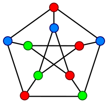 A proper vertex coloring of the Petersen graph with 3 colors, the minimum number possible.
Part - 2
Branch and bound
Branch and bound (BB, B&B, or BnB) is an algorithm design paradigm for discrete and combinatorial optimization problems, as well as mathematical optimization. A branch-and-bound algorithm consists of a systematic enumeration of candidate solutions by means of state space search: the set of candidate solutions is thought of as forming a rooted tree with the full set at the root. The algorithm explores branches of this tree, which represent subsets of the solution set. Before enumerating the candidate solutions of a branch, the branch is checked against upper and lower estimated bounds on the optimal solution, and is discarded if it cannot produce a better solution than the best one found so far by the algorithm.
The algorithm depends on the efficient estimation of the lower and upper bounds of a region/branch of the search space and approaches exhaustive enumeration as the size (n-dimensional volume) of the region tends to zero.
The method was first proposed by A. H. Land and A. G. Doig in 1960 for discrete programming, and has become the most commonly used tool for solving NP-hard optimization problems.The name "branch and bound" first occurred in the work of Little et al. on the traveling salesman problem.
Applications
This approach is used for a number of NP-hard problems
- Integer programming
- Nonlinear programming
- Travelling salesman problem (TSP)
- Quadratic assignment problem (QAP)
- Maximum satisfiability problem (MAX-SAT)
- Nearest neighbor search
- Flow shop scheduling
- Cutting stock problem
- False noise analysis (FNA)
- Computational phylogenetics
- Set inversion
- Parameter estimation
- 0/1 knapsack problem
- Feature selection in machine learning
- Structured prediction in computer vision
Branch-and-bound may also be a base of various heuristics. For example, one may wish to stop branching when the gap between the upper and lower bounds becomes smaller than a certain threshold. This is used when the solution is "good enough for practical purposes" and can greatly reduce the computations required. This type of solution is particularly applicable when the cost function used is noisy or is the result of statistical estimates and so is not known precisely but rather only known to lie within a range of values with a specific probability.
[https://en.wikipedia.org/wiki/Branch_and_bound]
Traveling Salesman Problem
Given a set of cities and distance between every pair of cities, the problem is to find the shortest possible tour that visits every city exactly once and returns to the starting point.

For example, consider the graph shown in figure on right side. A TSP tour in the graph is 0-1-3-2-0. The cost of the tour is 10+25+30+15 which is 80.
We have discussed following solutions
1) Naive and Dynamic Programming
2) Approximate solution using MST
1) Naive and Dynamic Programming
2) Approximate solution using MST
As seen in the previous articles, in Branch and Bound method, for current node in tree, we compute a bound on best possible solution that we can get if we down this node. If the bound on best possible solution itself is worse than current best (best computed so far), then we ignore the subtree rooted with the node.
Note that the cost through a node includes two costs.
1) Cost of reaching the node from the root (When we reach a node, we have this cost computed)
2) Cost of reaching an answer from current node to a leaf (We compute a bound on this cost to decide whether to ignore subtree with this node or not).
1) Cost of reaching the node from the root (When we reach a node, we have this cost computed)
2) Cost of reaching an answer from current node to a leaf (We compute a bound on this cost to decide whether to ignore subtree with this node or not).
- In cases of a maximization problem, an upper bound tells us the maximum possible solution if we follow the given node. For example in 0/1 knapsack we used Greedy approach to find an upper bound.
- In cases of a minimization problem, a lower bound tells us the minimum possible solution if we follow the given node. For example, in Job Assignment Problem, we get a lower bound by assigning least cost job to a worker.
In branch and bound, the challenging part is figuring out a way to compute a bound on best possible solution. Below is an idea used to compute bounds for Traveling salesman problem.
Cost of any tour can be written as below.
Cost of a tour T = (1/2) * ∑ (Sum of cost of two edges
                              adjacent to u and in the
                              tour T)
                   where u ∈ V
For every vertex u, if we consider two edges through it in T,
and sum their costs.  The overall sum for all vertices would
be twice of cost of tour T (We have considered every edge
twice.)

(Sum of two tour edges adjacent to u) >= (sum of minimum weight
                                          two edges adjacent to
                                          u)

Cost of any tour >=  1/2) * ∑ (Sum of cost of two minimum
                              weight edges adjacent to u)
                   where u ∈ V
For example, consider the above shown graph. Below are minimum cost two edges adjacent to every node.
Node  Least cost edges   Total cost
0  (0, 1), (0, 2)         25
1  (0, 1), (1, 3)         35
2 (0, 2), (2, 3)         45
3  (0, 3), (1, 3)         45

Thus a lower bound on the cost of any tour =
         1/2(25 + 35 + 45 + 45)
       = 75
Refer this for one more example.
Now we have an idea about computation of lower bound. Let us see how to how to apply it state space search tree. We start enumerating all possible nodes (preferably in lexicographical order)
1. The Root Node: Without loss of generality, we assume we start at vertex “0” for which the lower bound has been calculated above.
Dealing with Level 2: The next level enumerates all possible vertices we can go to (keeping in mind that in any path a vertex has to occur only once) which are, 1, 2, 3… n (Note that the graph is complete). Consider we are calculating for vertex 1, Since we moved from 0 to 1, our tour has now included the edge 0-1. This allows us to make necessary changes in the lower bound of the root.
Lower Bound for vertex 1 =
   Old lower bound - ((minimum edge cost of 0 +
                    minimum edge cost of 1) / 2)
                  + (edge cost 0-1)
How does it work? To include edge 0-1, we add the edge cost of 0-1, and subtract an edge weight such that the lower bound remains as tight as possible which would be the sum of the minimum edges of 0 and 1 divided by 2. Clearly, the edge subtracted can’t be smaller than this.
Dealing with other levels: As we move on to the next level, we again enumerate all possible vertices. For the above case going further after 1, we check out for 2, 3, 4, …n.
Consider lower bound for 2 as we moved from 1 to 1, we include the edge 1-2 to the tour and alter the new lower bound for this node.
Consider lower bound for 2 as we moved from 1 to 1, we include the edge 1-2 to the tour and alter the new lower bound for this node.
Lower bound(2) =
     Old lower bound - ((second minimum edge cost of 1 +
                         minimum edge cost of 2)/2)
                     + edge cost 1-2)
Note: The only change in the formula is that this time we have included second minimum edge cost for 1, because the minimum edge cost has already been subtracted in previous level.
// C++ program to solve Traveling Salesman Problem// using Branch and Bound.#include <bits/stdc++.h>using namespace std;const int N = 4;// final_path[] stores the final solution ie, the// path of the salesman.int final_path[N+1];// visited[] keeps track of the already visited nodes// in a particular pathbool visited[N];// Stores the final minimum weight of shortest tour.int final_res = INT_MAX;// Function to copy temporary solution to// the final solutionvoid copyToFinal(int curr_path[]){ for (int i=0; i<N; i++) final_path[i] = curr_path[i]; final_path[N] = curr_path[0];}// Function to find the minimum edge cost// having an end at the vertex iint firstMin(int adj[N][N], int i){ int min = INT_MAX; for (int k=0; k<N; k++) if (adj[i][k]<min && i != k) min = adj[i][k]; return min;}// function to find the second minimum edge cost// having an end at the vertex iint secondMin(int adj[N][N], int i){ int first = INT_MAX, second = INT_MAX; for (int j=0; j<N; j++) { if (i == j) continue; if (adj[i][j] <= first) { second = first; first = adj[i][j]; } else if (adj[i][j] <= second && adj[i][j] != first) second = adj[i][j]; } return second;}// function that takes as arguments:// curr_bound -> lower bound of the root node// curr_weight-> stores the weight of the path so far// level-> current level while moving in the search// space tree// curr_path[] -> where the solution is being stored which// would later be copied to final_path[]void TSPRec(int adj[N][N], int curr_bound, int curr_weight, int level, int curr_path[]){ // base case is when we have reached level N which // means we have covered all the nodes once if (level==N) { // check if there is an edge from last vertex in // path back to the first vertex if (adj[curr_path[level-1]][curr_path[0]] != 0) { // curr_res has the total weight of the // solution we got int curr_res = curr_weight + adj[curr_path[level-1]][curr_path[0]]; // Update final result and final path if // current result is better. if (curr_res < final_res) { copyToFinal(curr_path); final_res = curr_res; } } return; } // for any other level iterate for all vertices to // build the search space tree recursively for (int i=0; i<N; i++) { // Consider next vertex if it is not same (diagonal // entry in adjacency matrix and not visited // already) if (adj[curr_path[level-1]][i] != 0 && visited[i] == false) { int temp = curr_bound; curr_weight += adj[curr_path[level-1]][i]; // different computation of curr_bound for // level 2 from the other levels if (level==1) curr_bound -= ((firstMin(adj, curr_path[level-1]) + firstMin(adj, i))/2); else curr_bound -= ((secondMin(adj, curr_path[level-1]) + firstMin(adj, i))/2); // curr_bound + curr_weight is the actual lower bound // for the node that we have arrived on // If current lower bound < final_res, we need to explore // the node further if (curr_bound + curr_weight < final_res) { curr_path[level] = i; visited[i] = true; // call TSPRec for the next level TSPRec(adj, curr_bound, curr_weight, level+1, curr_path); } // Else we have to prune the node by resetting // all changes to curr_weight and curr_bound curr_weight -= adj[curr_path[level-1]][i]; curr_bound = temp; // Also reset the visited array memset(visited, false, sizeof(visited)); for (int j=0; j<=level-1; j++) visited[curr_path[j]] = true; } }}// This function sets up final_path[] void TSP(int adj[N][N]){ int curr_path[N+1]; // Calculate initial lower bound for the root node // using the formula 1/2 * (sum of first min + // second min) for all edges. // Also initialize the curr_path and visited array int curr_bound = 0; memset(curr_path, -1, sizeof(curr_path)); memset(visited, 0, sizeof(curr_path)); // Compute initial bound for (int i=0; i<N; i++) curr_bound += (firstMin(adj, i) + secondMin(adj, i)); // Rounding off the lower bound to an integer curr_bound = (curr_bound&1)? curr_bound/2 + 1 : curr_bound/2; // We start at vertex 1 so the first vertex // in curr_path[] is 0 visited[0] = true; curr_path[0] = 0; // Call to TSPRec for curr_weight equal to // 0 and level 1 TSPRec(adj, curr_bound, 0, 1, curr_path);}// Driver codeint main(){ //Adjacency matrix for the given graph int adj[N][N] = { {0, 10, 15, 20}, {10, 0, 35, 25}, {15, 35, 0, 30}, {20, 25, 30, 0} }; TSP(adj); printf("Minimum cost : %d\n", final_res); printf("Path Taken : "); for (int i=0; i<=N; i++) printf("%d ", final_path[i]); return 0;} |
Output :
Minimum cost : 80
Path Taken : 0 1 3 2 0
Time Complexity: The worst case complexity of Branch and Bound remains same as that of the Brute Force clearly because in worst case, we may never get a chance to prune a node. Whereas, in practice it performs very well depending on the different instance of the TSP. The complexity also depends on the choice of the bounding function as they are the ones deciding how many nodes to be pruned.
[http://www.geeksforgeeks.org/branch-bound-set-5-traveling-salesman-problem/]
Optimal Solution for TSP using Branch and Bound
Principle
Suppose it is required to minimize an objective function. Suppose that we have a method for getting a lower bound on the cost of any solution among those in the set of solutions represented by some subset. If the best solution found so far costs less than the lower bound for this subset, we need not explore this subset at all.
Let S be some subset of solutions. Let
| L(S) | = | a lower bound on the cost of | |
| Let C | = | cost of the best solution | |
| found so far |
| If C | there is no need to explore S because it does |
| not contain any better solution. | |
| If C > L(S), | then we need to explore S because it may |
| contain a better solution. |
A Lower Bound for a TSP
Note that:
Cost of any tour
= 

Now:
Now:
The sum of the two tour edges adjacent to a given vertex v
Therefore:

 |
| Node | Least cost edges | Total cost |
| a | (a, d), (a, b) | 5 |
| b | (a, b), (b, e) | 6 |
| c | (c, b), (c, a) | 8 |
| d | (d, a), (d, c) | 7 |
| e | (e, b), (e, f) | 9 |
Thus a lower bound on the cost of any tour
 |
- Suppose we want a lower bound on the cost of a subset of tours defined by some node in the search tree.
- These constraints alter our choices for the two lowest cost edges at each node.
- Each time we branch, by considering the two children of a node, we try to infer additional decisions regarding which edges must be included or excluded from tours represented by those nodes. The rules we use for these inferences are:
- 1.
- If excluding (x, y) would make it impossible for x or y to have as many as two adjacent edges in the tour, then (x, y) must be included.
- 2.
- If including (x, y) would cause x or y to have more than two edges adjacent in the tour, or would complete a non-tour cycle with edges already included, then (x, y) must be excluded.
- See Figure 8.19.
- When we branch, after making what inferences we can, we compute lower bounds for both children. If the lower bound for a child is as high or higher than the lowest cost found so far, we can ``prune'' that child and need not consider or construct its descendants.
- If neither child can be pruned, we shall, as a heuristic, consider first the child with the smaller lower bound. After considering one child, we must consider again whether its sibling can be pruned, since a new best solution may have been found.
In the above solution tree, each node represents tours defined by a set of edges that must be in the tour and a set of edges that may not be in the tour.
e.g., if we are constrained to include edge (a, e), and exclude (b, c), then we will have to select the two lowest cost edges as follows:
| a | (a, d), (a, e) | 9 |
| b | (a, b), (b, e) | 6 |
| c | (a, c), (c, d) | 9 |
| d | (a, d), (c, d) | 7 |
| e | (a, e), (b, e) | 10 |
Interestingly, there are situations where the lower bound for a node n is lower than the best solution so far, yet both children of n can be pruned because their lower bounds exceed the cost of the best solution so far.
 |
[http://lcm.csa.iisc.ernet.in/dsa/node187.html]
LOWER BOUND THEORY
The goal of a branch-and-bound algorithm is to find a value x that maximizes or minimizes the value of a real-valued function f(x), called an objective function, among some set S of admissible, or candidate solutions. The set S is called the search space, or feasible region. The rest of this section assumes that minimization of f(x) is desired; this assumption comes without loss of generality, since one can find the maximum value of f(x) by finding the minimum of g(x) = −f(x). A B&B algorithm operates according to two principles:
- It recursively splits the search space into smaller spaces, then minimizing f(x) on these smaller spaces; the splitting is called branching.
- Branching alone would amount to brute-force enumeration of candidate solutions and testing them all. To improve on the performance of brute-force search, a B&B algorithm keeps track of bounds on the minimum that it is trying to find, and uses these bounds to "prune" the search space, eliminating candidate solutions that it can prove will not contain an optimal solution.
Turning these principles into a concrete algorithm for a specific optimization problem requires some kind of data structure that represents sets of candidate solutions. Such a representation is called an instance of the problem. Denote the set of candidate solutions of an instance I by SI. The instance representation has to come with three operations:
- branch(I) produces two or more instances that each represent a subset of SI. (Typically, the subsets are disjoint to prevent the algorithm from visiting the same candidate solution twice, but this is not required. The only requirement for a correct B&B algorithm is that the optimal solution among SI is contained in at least one of the subsets.[5])
- bound(I) computes a lower bound on the value of any candidate solution in the space represented by I, that is, bound(I) ≤ f(x) for all x in SI.
- solution(I) determines whether I represents a single candidate solution. (Optionally, if it does not, the operation may choose to return some feasible solution from among SI.[5])
Using these operations, a B&B algorithm performs a top-down recursive search through the tree of instances formed by the branch operation. Upon visiting an instance I, it checks whether bound(I) is greater than the upper bound for some other instance that it already visited; if so, I may be safely discarded from the search and the recursion stops. This pruning step is usually implemented by maintaining a global variable that records the minimum upper bound seen among all instances examined so far.
Generic version
The following is the skeleton of a generic branch and bound algorithm for minimizing an arbitrary objective function f. To obtain an actual algorithm from this, one requires a bounding function g, that computes lower bounds of f on nodes of the search tree, as well as a problem-specific branching rule.
- Using a heuristic, find a solution xh to the optimization problem. Store its value, B = f(xh). (If no heuristic is available, set B to infinity.) B will denote the best solution found so far, and will be used as an upper bound on candidate solutions.
- Initialize a queue to hold a partial solution with none of the variables of the problem assigned.
- Loop until the queue is empty:
- Take a node N off the queue.
- If N represents a single candidate solution x and f(x) < B, then x is the best solution so far. Record it and set B ← f(x).
- Else, branch on N to produce new nodes Ni. For each of these:
- If g(Ni) > B, do nothing; since the lower bound on this node is greater than the upper bound of the problem, it will never lead to the optimal solution, and can be discarded.
- Else, store Ni on the queue.
Several different queue data structures can be used. A stack (LIFO queue) will yield a depth-first algorithm. A best-first branch and bound algorithm can be obtained by using a priority queue that sorts nodes on their g-value. The depth-first variant is recommended when no good heuristic is available for producing an initial solution, because it quickly produces full solutions, and therefore upper bounds.
Improvements
When is a vector of , branch and bound algorithms can be combined with interval analysis and contractor techniques in order to provide guaranteed enclosures of the global minimum.


Backtracking
Backtracking is a general algorithm for finding all (or some) solutions to some computational problems, notably constraint satisfaction problems, that incrementally builds candidates to the solutions, and abandons each partial candidate c ("backtracks") as soon as it determines that c cannot possibly be completed to a valid solution.
The classic textbook example of the use of backtracking is the eight queens puzzle, that asks for all arrangements of eight chess queens on a standard chessboard so that no queen attacks any other. In the common backtracking approach, the partial candidates are arrangements of k queens in the first k rows of the board, all in different rows and columns. Any partial solution that contains two mutually attacking queens can be abandoned.
Backtracking can be applied only for problems which admit the concept of a "partial candidate solution" and a relatively quick test of whether it can possibly be completed to a valid solution. It is useless, for example, for locating a given value in an unordered table. When it is applicable, however, backtracking is often much faster than brute force enumeration of all complete candidates, since it can eliminate a large number of candidates with a single test.
Backtracking is an important tool for solving constraint satisfaction problems, such as crosswords, verbal arithmetic, Sudoku, and many other puzzles. It is often the most convenient (if not the most efficient) technique for parsing, for the knapsack problem and other combinatorial optimization problems. It is also the basis of the so-called logic programming languages such as Icon, Planner and Prolog.
Backtracking depends on user-given "black box procedures" that define the problem to be solved, the nature of the partial candidates, and how they are extended into complete candidates. It is therefore a metaheuristic rather than a specific algorithm – although, unlike many other meta-heuristics, it is guaranteed to find all solutions to a finite problem in a bounded amount of time.
The term "backtrack" was coined by American mathematician D. H. Lehmer in the 1950s.The pioneer string-processing language SNOBOL (1962) may have been the first to provide a built-in general backtracking facility.
[https://en.wikipedia.org/wiki/Backtracking]
Backtracking
- It is used to find all possible solutions available to a problem.
- It traverses the state space tree by DFS(Depth First Search) manner.
- It realizes that it has made a bad choice & undoes the last choice by backing up.
- It searches the state space tree until it has found a solution.
- It involves feasibility function.
Branch-and-Bound
- It is used to solve optimization problem.
- It may traverse the tree in any manner, DFS or BFS.
- It realizes that it already has a better optimal solution that the pre-solution leads to so it abandons that pre-solution.
- It completely searches the state space tree to get optimal solution.
- It involves a bounding function.
[http://stackoverflow.com/questions/30025421/difference-between-backtracking-and-branch-and-bound]
0/1 Knapsack
Branch and bound is an algorithm design paradigm which is generally used for solving combinatorial optimization problems. These problems typically exponential in terms of time complexity and may require exploring all possible permutations in worst case. Branch and Bound solve these problems relatively quickly.
Let us consider below 0/1 Knapsack problem to understand Branch and Bound.
Given two integer arrays val[0..n-1] and wt[0..n-1] that represent values and weights associated with n items respectively. Find out the maximum value subset of val[] such that sum of the weights of this subset is smaller than or equal to Knapsack capacity W.
Let us explore all approaches for this problem.
- A Greedy approach is to pick the items in decreasing order of value per unit weight. The Greedy approach works only for fractional knapsack problem and may not produce correct result for 0/1 knapsack.
- We can use Dynamic Programming (DP) for 0/1 Knapsack problem. In DP, we use a 2D table of size n x W. The DP Solution doesn’t work if item weights are not integers.
- Since DP solution doesn’t alway work, a solution is to use Brute Force. With n items, there are 2n solutions to be generated, check each to see if they satisfy the constraint, save maximum solution that satisfies constraint. This solution can be expressed as tree.
- We can use Backtracking to optimize the Brute Force solution. In the tree representation, we can do DFS of tree. If we reach a point where a solution no longer is feasible, there is no need to continue exploring. In the given example, backtracking would be much more effective if we had even more items or a smaller knapsack capacity.


The backtracking based solution works better than brute force by ignoring infeasible solutions. We can do better (than backtracking) if we know a bound on best possible solution subtree rooted with every node. If the best in subtree is worse than current best, we can simply ignore this node and its subtrees. So we compute bound (best solution) for every node and compare the bound with current best solution before exploring the node.
Example bounds used in below diagram are, A down can give $315, B down can $275, C down can $225, D down can $125 and E down can $30. In the next article, we have discussed the process to get these bounds.

Branch and bound is very useful technique for searching a solution but in worst case, we need to fully calculate the entire tree. At best, we only need to fully calculate one path through the tree and prune the rest of it.
[http://www.geeksforgeeks.org/branch-and-bound-set-1-introduction-with-01-knapsack/]
N Queen Problem)
The N queens puzzle is the problem of placing N chess queens on an N×N chessboard so that no two queens threaten each other. Thus, a solution requires that no two queens share the same row, column, or diagonal.
For example, below is one of the solution for famous 8 Queen problem.

Backtracking Algorithm for N-Queen is already discussed here. In backtracking solution we backtrack when we hit a dead end. In Branch and Bound solution, after building a partial solution, we figure out that there is no point going any deeper as we are going to hit a dead end.
Let’s begin by describing backtracking solution. “The idea is to place queens one by one in different columns, starting from the leftmost column. When we place a queen in a column, we check for clashes with already placed queens. In the current column, if we find a row for which there is no clash, we mark this row and column as part of the solution. If we do not find such a row due to clashes, then we backtrack and return false.”

- For the 1st Queen, there are total 8 possibilities as we can place 1st Queen in any row of first column. Let’s place Queen 1 on row 3.
- After placing 1st Queen, there are 7 possibilities left for the 2nd Queen. But wait, we don’t really have 7 possibilities. We cannot place Queen 2 on rows 2, 3 or 4 as those cells are under attack from Queen 1. So, Queen 2 has only 8 – 3 = 5 valid positions left.
- After picking a position for Queen 2, Queen 3 has even fewer options as most of the cells in its column are under attack from the first 2 Queens.
We need to figure out an efficient way of keeping track of which cells are under attack. In previous solution we kept an 8-by-8 Boolean matrix and update it each time we placed a queen, but that required linear time to update as we need to check for safe cells.
Basically, we have to ensure 4 things:
1. No two queens share a column.
2. No two queens share a row.
3. No two queens share a top-right to left-bottom diagonal.
4. No two queens share a top-left to bottom-right diagonal.
1. No two queens share a column.
2. No two queens share a row.
3. No two queens share a top-right to left-bottom diagonal.
4. No two queens share a top-left to bottom-right diagonal.
Number 1 is automatic because of the way we store the solution. For number 2, 3 and 4, we can perform updates in O(1) time. The idea is to keep three Boolean arrays that tell us which rows and which diagonals are occupied.
Lets do some pre-processing first. Let’s create two N x N matrix one for / diagonal and other one for \ diagonal. Let’s call them slashCode and backslashCode respectively. The trick is to fill them in such a way that two queens sharing a same /diagonal will have the same value in matrix slashCode, and if they share same \diagonal, they will have the same value in backslashCode matrix.
For an N x N matrix, fill slashCode and backslashCode matrix using below formula –
slashCode[row][col] = row + col
backslashCode[row][col] = row – col + (N-1)
backslashCode[row][col] = row – col + (N-1)
Using above formula will result in below matrices


The ‘N – 1’ in the backslash code is there to ensure that the codes are never negative because we will be using the codes as indices in an array.
Now before we place queen i on row j, we first check whether row j is used (use an array to store row info). Then we check whether slash code ( j + i ) or backslash code ( j – i + 7 ) are used (keep two arrays that will tell us which diagonals are occupied). If yes, then we have to try a different location for queen i. If not, then we mark the row and the two diagonals as used and recurse on queen i + 1. After the recursive call returns and before we try another position for queen i, we need to reset the row, slash code and backslash code as unused again, like in the code from the previous notes.
Below is C++ implementation of above idea –
/* C++ program to solve N Queen Problem using Branch and Bound */#include<stdio.h>#include<string.h>#define N 8/* A utility function to print solution */void printSolution(int board[N][N]){ for (int i = 0; i < N; i++) { for (int j = 0; j < N; j++) printf("%2d ", board[i][j]); printf("\n"); }}/* A Optimized function to check if a queen canbe placed on board[row][col] */bool isSafe(int row, int col, int slashCode[N][N], int backslashCode[N][N], bool rowLookup[], bool slashCodeLookup[], bool backslashCodeLookup[] ){ if (slashCodeLookup[slashCode[row][col]] || backslashCodeLookup[backslashCode[row][col]] || rowLookup[row]) return false; return true;}/* A recursive utility function to solve N Queen problem */bool solveNQueensUtil(int board[N][N], int col, int slashCode[N][N], int backslashCode[N][N], bool rowLookup[N], bool slashCodeLookup[], bool backslashCodeLookup[] ){ /* base case: If all queens are placed then return true */ if (col >= N) return true; /* Consider this column and try placing this queen in all rows one by one */ for (int i = 0; i < N; i++) { /* Check if queen can be placed on board[i][col] */ if ( isSafe(i, col, slashCode, backslashCode, rowLookup, slashCodeLookup, backslashCodeLookup) ) { /* Place this queen in board[i][col] */ board[i][col] = 1; rowLookup[i] = true; slashCodeLookup[slashCode[i][col]] = true; backslashCodeLookup[backslashCode[i][col]] = true; /* recur to place rest of the queens */ if ( solveNQueensUtil(board, col + 1, slashCode, backslashCode, rowLookup, slashCodeLookup, backslashCodeLookup) ) return true; /* If placing queen in board[i][col] doesn't lead to a solution, then backtrack */ /* Remove queen from board[i][col] */ board[i][col] = 0; rowLookup[i] = false; slashCodeLookup[slashCode[i][col]] = false; backslashCodeLookup[backslashCode[i][col]] = false; } } /* If queen can not be place in any row in this colum col then return false */ return false;}/* This function solves the N Queen problem usingBranch and Bound. It mainly uses solveNQueensUtil() tosolve the problem. It returns false if queenscannot be placed, otherwise return true andprints placement of queens in the form of 1s.Please note that there may be more than onesolutions, this function prints one of thefeasible solutions.*/bool solveNQueens(){ int board[N][N]; memset(board, 0, sizeof board); // helper matrices int slashCode[N][N]; int backslashCode[N][N]; // arrays to tell us which rows are occupied bool rowLookup[N] = {false}; //keep two arrays to tell us which diagonals are occupied bool slashCodeLookup[2*N - 1] = {false}; bool backslashCodeLookup[2*N - 1] = {false}; // initalize helper matrices for (int r = 0; r < N; r++) for (int c = 0; c < N; c++) slashCode[r] = r + c, backslashCode[r] = r - c + 7; if (solveNQueensUtil(board, 0, slashCode, backslashCode, rowLookup, slashCodeLookup, backslashCodeLookup) == false ) { printf("Solution does not exist"); return false; } // solution found printSolution(board); return true;}// driver program to test above functionint main(){ solveNQueens(); return 0;} |
Output :
 1  0  0  0  0  0  0  0
 0  0  0  0  0  0  1  0
 0  0  0  0  1  0  0  0
 0  0  0  0  0  0  0  1
 0  1  0  0  0  0  0  0
 0  0  0  1  0  0  0  0
 0  0  0  0  0  1  0  0
 0  0  1  0  0  0  0  0
Performance:
When run on local machines for N = 32, the backtracking solution took 659.68 seconds while above branch and bound solution took only 119.63 seconds. The difference will be even huge for larger values of N.
When run on local machines for N = 32, the backtracking solution took 659.68 seconds while above branch and bound solution took only 119.63 seconds. The difference will be even huge for larger values of N.

[http://www.geeksforgeeks.org/branch-and-bound-set-4-n-queen-problem/]
Subset sum problem
In computer science, the subset sum problem is an important problem in complexity theory and cryptography. The problem is this: given a set (or multiset) of integers, is there a non-empty subset whose sum is zero? For example, given the set {−7, −3, −2, 5, 8}, the answer is yes because the subset {−3, −2, 5} sums to zero. The problem is NP-complete.
An equivalent problem is this: given a set of integers and an integer s, does any non-empty subset sum to s? Subset sum can also be thought of as a special case of the knapsack problem. One interesting special case of subset sum is the partition problem, in which s is half of the sum of all elements in the set.
Complexity
The complexity of the subset sum problem can be viewed as depending on two parameters, N, the number of decision variables, and P, the precision of the problem (stated as the number of binary place values that it takes to state the problem). (Note: here the letters N and P mean something different from what they mean in the NP class of problems.)
The complexity of the best known algorithms is exponential in the smaller of the two parameters N and P. Thus, the problem is most difficult if N and P are of the same order. It only becomes easy if either N or P becomes very small.
If N (the number of variables) is small, then an exhaustive search for the solution is practical. If P (the number of place values) is a small fixed number, then there are dynamic programming algorithms that can solve it exactly.
Efficient algorithms for both small N and small P cases are given below.
Exponential time algorithm[edit]
There are several ways to solve subset sum in time exponential in N. The most naïve algorithm would be to cycle through all subsets of N numbers and, for every one of them, check if the subset sums to the right number. The running time is of order O(2NN), since there are 2N subsets and, to check each subset, we need to sum at most N elements.
A better exponential time algorithm is known which runs in time O(2N/2). The algorithm splits arbitrarily the N elements into two sets of N/2 each. For each of these two sets, it stores a list of the sums of all 2N/2possible subsets of its elements. Each of these two lists is then sorted. Using a standard comparison sorting algorithm for this step would take time O(2N/2N). However, given a sorted list of sums for k elements, the list can be expanded to two sorted lists with the introduction of a (k + 1)st element, and these two sorted lists can be merged in time O(2k). Thus, each list can be generated in sorted form in time O(2N/2). Given the two sorted lists, the algorithm can check if an element of the first array and an element of the second array sum up to s in time O(2N/2). To do that, the algorithm passes through the first array in decreasing order (starting at the largest element) and the second array in increasing order (starting at the smallest element). Whenever the sum of the current element in the first array and the current element in the second array is more than s, the algorithm moves to the next element in the first array. If it is less than s, the algorithm moves to the next element in the second array. If two elements with sum s are found, it stops. Horowitz and Sahni first published this algorithm in a technical report in 1972.
Pseudo-polynomial time dynamic programming solution
The problem can be solved in pseudo-polynomial time using dynamic programming. Suppose the sequence is
- x1, ..., xN
and we wish to determine if there is a nonempty subset which sums to zero. Define the boolean-valued function Q(i, s) to be the value (true or false) of
- "there is a nonempty subset of x1, ..., xi which sums to s".
Thus, the solution to the problem "Given a set of integers, is there a non-empty subset whose sum is zero?" is the value of Q(N, 0).
Let A be the sum of the negative values and B the sum of the positive values. Clearly, Q(i, s) = false, if s < A or s > B. So these values do not need to be stored or computed.
Create an array to hold the values Q(i, s) for 1 ≤ i ≤ N and A ≤ s ≤ B.
The array can now be filled in using a simple recursion. Initially, for A ≤ s ≤ B, set
- Q(1, s) := (x1 == s)
where == is a boolean function that returns true if x1 is equal to s, false otherwise.
Then, for i = 2, …, N, set
- Q(i, s) := Q(i − 1, s) or (xi == s) or Q(i − 1, s − xi), for A ≤ s ≤ B.
For each assignment, the values of Q on the right side are already known, either because they were stored in the table for the previous value of i or because Q(i − 1,s − xi) = false if s − xi < A or s − xi > B. Therefore, the total number of arithmetic operations is O(N(B − A)). For example, if all the values are O(Nk) for some k, then the time required is O(Nk+2).
This algorithm is easily modified to return the subset with sum 0 if there is one.
The dynamic programming solution has runtime of where is the sum we want to find in set of numbers. This solution does not count as polynomial time in complexity theory because B − A is not polynomial in the size of the problem, which is the number of bits used to represent it. This algorithm is polynomial in the values of A and B, which are exponential in their numbers of bits.
 where
where  is the sum we want to find in set of
  numbers. This solution does not count as polynomial time in complexity theory because
For the case that each xi is positive and bounded by a fixed constant C, found a linear time algorithm having time complexity O(NC) (note that this is for the version of the problem where the target sum is not necessarily zero, otherwise the problem would be trivial). In 2015, Koiliaris and Xu found the algorithm for the subset sum problem where is the sum we need to find.

Polynomial time approximate algorithm
An approximate version of the subset sum would be: given a set of N numbers x1, x2, ..., xN and a number s, output
- yes, if there is a subset that sums up to s;
- no, if there is no subset summing up to a number between (1 − c)s and s for some small c > 0;
- any answer, if there is a subset summing up to a number between (1 − c)s and s but no subset summing up to s.
If all numbers are non-negative, the approximate subset sum is solvable in time polynomial in N and 1/c.
The solution for subset sum also provides the solution for the original subset sum problem in the case where the numbers are small (again, for nonnegative numbers). If any sum of the numbers can be specified with at most P bits, then solving the problem approximately with c = 2−P is equivalent to solving it exactly. Then, the polynomial time algorithm for approximate subset sum becomes an exact algorithm with running time polynomial in N and 2P (i.e., exponential in P).
The algorithm for the approximate subset sum problem is as follows:
initialize a list S to contain one element 0.for each i from 1 to N dolet T be a list consisting of xi + y, for all y in Slet U be the union of T and Ssort Umake S emptylet y be the smallest element of Uadd y to Sfor each element z of U in increasing order do//trim the list by eliminating numbers close to one another//and throw out elements greater than sif y + cs/N < z ≤ s, set y = z and add z to Sif S contains a number between (1 − c)s and s, output yes, otherwise no
The algorithm is polynomial time because the lists S, T and U always remain of size polynomial in N and 1/c and, as long as they are of polynomial size, all operations on them can be done in polynomial time. The size of lists is kept polynomial by the trimming step, in which we only include a number z into S if it is greater than the previous one by cs/N and not greater than s.
This step ensures that each element in S is smaller than the next one by at least cs/N and do not contain elements greater than s. Any list with that property consists of no more than N/c elements.
The algorithm is correct because each step introduces an additive error of at most cs/N and N steps together introduce the error of at most cs.
Graph coloring
In graph theory, graph coloring is a special case of graph labeling; it is an assignment of labels traditionally called "colors" to elements of a graph subject to certain constraints. In its simplest form, it is a way of coloring the vertices of a graph such that no two adjacent vertices share the same color; this is called a vertex coloring. Similarly, an edge coloring assigns a color to each edge so that no two adjacent edges share the same color, and a face coloring of a planar graph assigns a color to each face or region so that no two faces that share a boundary have the same color.
Vertex coloring is the starting point of the subject, and other coloring problems can be transformed into a vertex version. For example, an edge coloring of a graph is just a vertex coloring of its line graph, and a face coloring of a plane graph is just a vertex coloring of its dual. However, non-vertex coloring problems are often stated and studied as is. That is partly for perspective, and partly because some problems are best studied in non-vertex form, as for instance is edge coloring.
The convention of using colors originates from coloring the countries of a map, where each face is literally colored. This was generalized to coloring the faces of a graph embedded in the plane. By planar duality it became coloring the vertices, and in this form it generalizes to all graphs. In mathematical and computer representations, it is typical to use the first few positive or nonnegative integers as the "colors". In general, one can use any finite set as the "color set". The nature of the coloring problem depends on the number of colors but not on what they are.
Graph coloring enjoys many practical applications as well as theoretical challenges. Beside the classical types of problems, different limitations can also be set on the graph, or on the way a color is assigned, or even on the color itself. It has even reached popularity with the general public in the form of the popular number puzzle Sudoku. Graph coloring is still a very active field of research.

[https://en.wikipedia.org/wiki/Graph_coloring]
[https://en.wikipedia.org/wiki/Subset_sum_problem#Exponential_time_algorithm]