Design and Analysis of Algorithms 2

Unit - IPart - 2Divide and Conquer (or Rule)

"The policy of maintaining control over one's subordinates or opponents by encouraging dissent between them, thereby preventing them from uniting in opposition."

In computer science, divide and conquer (D&C) is an algorithm design paradigm based on multi-branched recursion. A divide and conquer algorithm works by recursively breaking down a problem into two or more sub-problems of the same or related type, until these become simple enough to be solved directly. The solutions to the sub-problems are then combined to give a solution to the original problem.

This divide and conquer technique is the basis of efficient algorithms for all kinds of problems, such as sorting (e.g., quicksort, merge sort), multiplying large numbers (e.g. the Karatsuba algorithm), finding the closest pair of points, syntactic analysis (e.g., top-down parsers), and computing the discrete Fourier transform (FFTs).

Understanding and designing D&C algorithms is a complex skill that requires a good understanding of the nature of the underlying problem to be solved. As when proving a theorem by induction, it is often necessary to replace the original problem with a more general or complicated problem in order to initialize the recursion, and there is no systematic method for finding the proper generalization. These D&C complications are seen when optimizing the calculation of a Fibonacci number with efficient double recursion.

The correctness of a divide and conquer algorithm is usually proved by mathematical induction, and its computational cost is often determined by solving recurrence relations.

In divide and conquer approach, the problem in hand, is divided into smaller sub-problems and then each problem is solved independently. When we keep on dividing the subproblems into even smaller sub-problems, we may eventually reach a stage where no more division is possible. Those "atomic" smallest possible sub-problem (fractions) are solved. The solution of all sub-problems is finally merged in order to obtain the solution of an original problem.

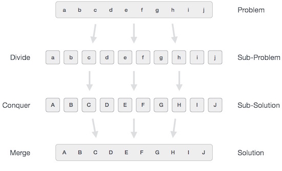Broadly, we can understand divide-and-conquer approach in a three-step process.

Divide/Break

This step involves breaking the problem into smaller sub-problems. Sub-problems should represent a part of the original problem. This step generally takes a recursive approach to divide the problem until no sub-problem is further divisible. At this stage, sub-problems become atomic in nature but still represent some part of the actual problem.

Conquer/Solve

This step receives a lot of smaller sub-problems to be solved. Generally, at this level, the problems are considered 'solved' on their own.

Merge/Combine

When the smaller sub-problems are solved, this stage recursively combines them until they formulate a solution of the original problem. This algorithmic approach works recursively and conquer & merge steps works so close that they appear as one.

Examples

The following computer algorithms are based on divide-and-conquer programming approach −

• Merge Sort
• Quick Sort
• Binary Search
• Strassen's Matrix Multiplication
• Closest pair (points)

There are various ways available to solve any computer problem, but the mentioned are a good example of divide and conquer approach.

Advantages

Solving difficult problems

Divide and conquer is a powerful tool for solving conceptually difficult problems: all it requires is a way of breaking the problem into sub-problems, of solving the trivial cases and of combining sub-problems to the original problem. Similarly, decrease and conquer only requires reducing the problem to a single smaller problem, such as the classic Tower of Hanoi puzzle, which reduces moving a tower of height n to moving a tower of height n − 1.

Algorithm efficiency

The divide-and-conquer paradigm often helps in the discovery of efficient algorithms. It was the key, for example, to Karatsuba's fast multiplication method, the quicksort and mergesort algorithms, the Strassen algorithm for matrix multiplication, and fast Fourier transforms.

In all these examples, the D&C approach led to an improvement in the asymptotic cost of the solution. For example, if (a) the base cases have constant-bounded size, the work of splitting the problem and combining the partial solutions is proportional to the problem's size n, and (b) there is a bounded number p of subproblems of size ~ n/p at each stage, then the cost of the divide-and-conquer algorithm will be O(n logpn).

Parallelism

Divide and conquer algorithms are naturally adapted for execution in multi-processor machines, especially shared-memory systems where the communication of data between processors does not need to be planned in advance, because distinct sub-problems can be executed on different processors.

Memory access

Divide-and-conquer algorithms naturally tend to make efficient use of memory caches. The reason is that once a sub-problem is small enough, it and all its sub-problems can, in principle, be solved within the cache, without accessing the slower main memory. An algorithm designed to exploit the cache in this way is called cache-oblivious, because it does not contain the cache size as an explicit parameter.[8] Moreover, D&C algorithms can be designed for important algorithms (e.g., sorting, FFTs, and matrix multiplication) to be optimal cache-oblivious algorithms–they use the cache in a probably optimal way, in an asymptotic sense, regardless of the cache size. In contrast, the traditional approach to exploiting the cache is blocking, as in loop nest optimization, where the problem is explicitly divided into chunks of the appropriate size—this can also use the cache optimally, but only when the algorithm is tuned for the specific cache size(s) of a particular machine.

The same advantage exists with regards to other hierarchical storage systems, such as NUMA or virtual memory, as well as for multiple levels of cache: once a sub-problem is small enough, it can be solved within a given level of the hierarchy, without accessing the higher (slower) levels.

Roundoff control

In computations with rounded arithmetic, e.g. with floating point numbers, a divide-and-conquer algorithm may yield more accurate results than a superficially equivalent iterative method. For example, one can add N numbers either by a simple loop that adds each datum to a single variable, or by a D&C algorithm called pairwise summation that breaks the data set into two halves, recursively computes the sum of each half, and then adds the two sums. While the second method performs the same number of additions as the first, and pays the overhead of the recursive calls, it is usually more accurate.

Implementation issues

Recursion

Divide-and-conquer algorithms are naturally implemented as recursive procedures. In that case, the partial sub-problems leading to the one currently being solved are automatically stored in the procedure call stack. A recursive function is a function that calls itself within its definition.

Explicit stack

Divide and conquer algorithms can also be implemented by a non-recursive program that stores the partial sub-problems in some explicit data structure, such as a stack, queue, or priority queue. This approach allows more freedom in the choice of the sub-problem that is to be solved next, a feature that is important in some applications — e.g. in breadth-first recursion and the branch and bound method for function optimization. This approach is also the standard solution in programming languages that do not provide support for recursive procedures.

Stack size

In recursive implementations of D&C algorithms, one must make sure that there is sufficient memory allocated for the recursion stack, otherwise the execution may fail because of stack overflow. Fortunately, D&C algorithms that are time-efficient often have relatively small recursion depth. For example, the quicksort algorithm can be implemented so that it never requires more than {\displaystyle \log _{2}n} \log _{2}n nested recursive calls to sort {\displaystyle n} n items.

Stack overflow may be difficult to avoid when using recursive procedures, since many compilers assume that the recursion stack is a contiguous area of memory, and some allocate a fixed amount of space for it. Compilers may also save more information in the recursion stack than is strictly necessary, such as return address, unchanging parameters, and the internal variables of the procedure. Thus, the risk of stack overflow can be reduced by minimizing the parameters and internal variables of the recursive procedure, or by using an explicit stack structure.

Choosing the base cases

In any recursive algorithm, there is considerable freedom in the choice of the base cases, the small subproblems that are solved directly in order to terminate the recursion.

Choosing the smallest or simplest possible base cases is more elegant and usually leads to simpler programs, because there are fewer cases to consider and they are easier to solve. For example, an FFT algorithm could stop the recursion when the input is a single sample, and the quicksort list-sorting algorithm could stop when the input is the empty list; in both examples there is only one base case to consider, and it requires no processing.

On the other hand, efficiency often improves if the recursion is stopped at relatively large base cases, and these are solved non-recursively, resulting in a hybrid algorithm. This strategy avoids the overhead of recursive calls that do little or no work, and may also allow the use of specialized non-recursive algorithms that, for those base cases, are more efficient than explicit recursion. A general procedure for a simple hybrid recursive algorithm is short-circuiting the base case, also known as arm's-length recursion. In this case whether the next step will result in the base case is checked before the function call, avoiding an unnecessary function call. For example, in a tree, rather than recursing to a child node and then checking if it is null, checking null before recursing; this avoids half the function calls in some algorithms on binary trees. Since a D&C algorithm eventually reduces each problem or sub-problem instance to a large number of base instances, these often dominate the overall cost of the algorithm, especially when the splitting/joining overhead is low. Note that these considerations do not depend on whether recursion is implemented by the compiler or by an explicit stack.

Thus, for example, many library implementations of quicksort will switch to a simple loop-based insertion sort (or similar) algorithm once the number of items to be sorted is sufficiently small. Note that, if the empty list were the only base case, sorting a list with n entries would entail maximally n quicksort calls that would do nothing but return immediately. Increasing the base cases to lists of size 2 or less will eliminate most of those do-nothing calls, and more generally a base case larger than 2 is typically used to reduce the fraction of time spent in function-call overhead or stack manipulation.

Alternatively, one can employ large base cases that still use a divide-and-conquer algorithm, but implement the algorithm for predetermined set of fixed sizes where the algorithm can be completely unrolled into code that has no recursion, loops, or conditionals (related to the technique of partial evaluation). For example, this approach is used in some efficient FFT implementations, where the base cases are unrolled implementations of divide-and-conquer FFT algorithms for a set of fixed sizes. Source code generation methods may be used to produce the large number of separate base cases desirable to implement this strategy efficiently.

The generalized version of this idea is known as recursion "unrolling" or "coarsening" and various techniques have been proposed for automating the procedure of enlarging the base case.

Sharing repeated subproblems

For some problems, the branched recursion may end up evaluating the same sub-problem many times over. In such cases it may be worth identifying and saving the solutions to these overlapping subproblems, a technique commonly known as memoization. Followed to the limit, it leads to bottom-up divide-and-conquer algorithms such as dynamic programming and chart parsing.

Binary Search

Binary search is a fast search algorithm with run-time complexity of Ο(log n). This search algorithm works on the principle of divide and conquer. For this algorithm to work properly, the data collection should be in the sorted form.

Binary search looks for a particular item by comparing the middle most item of the collection. If a match occurs, then the index of item is returned. If the middle item is greater than the item, then the item is searched in the sub-array to the left of the middle item. Otherwise, the item is searched for in the sub-array to the right of the middle item. This process continues on the sub-array as well until the size of the subarray reduces to zero.

How Binary Search Works?

For a binary search to work, it is mandatory for the target array to be sorted. We shall learn the process of binary search with a pictorial example. The following is our sorted array and let us assume that we need to search the location of value 31 using binary search.

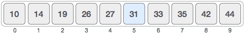
First, we shall determine half of the array by using this formula −

mid = low + (high - low) / 2

Here it is, 0 + (9 - 0 ) / 2 = 4 (integer value of 4.5). So, 4 is the mid of the array.

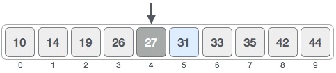
Now we compare the value stored at location 4, with the value being searched, i.e. 31. We find that the value at location 4 is 27, which is not a match. As the value is greater than 27 and we have a sorted array, so we also know that the target value must be in the upper portion of the array.

We change our low to mid + 1 and find the new mid value again.

low = mid + 1
mid = low + (high - low) / 2

Our new mid is 7 now. We compare the value stored at location 7 with our target value 31.

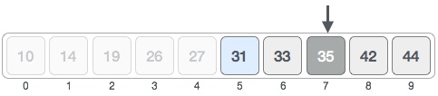
The value stored at location 7 is not a match, rather it is less than what we are looking for. So, the value must be in the lower part from this location.

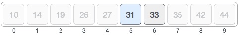
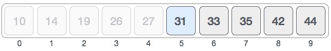
Hence, we calculate the mid again. This time it is 5.

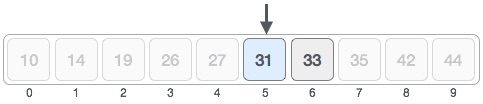
We compare the value stored at location 5 with our target value. We find that it is a match.

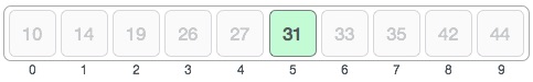
We conclude that the target value 31 is stored at location 5.

Binary search halves the searchable items and thus reduces the count of comparisons to be made to very less numbers.

Pseudocode

The pseudocode of binary search algorithms should look like this −

Procedure binary_search
   A ← sorted array
   n ← size of array
   x ← value to be searched

   Set lowerBound = 1
   Set upperBound = n 

   while x not found
      if upperBound < lowerBound 
         EXIT: x does not exists.
   
      set midPoint = lowerBound + ( upperBound - lowerBound ) / 2
      
      if A[midPoint] < x
         set lowerBound = midPoint + 1
         
      if A[midPoint] > x
         set upperBound = midPoint - 1 

      if A[midPoint] = x 
         EXIT: x found at location midPoint

   end while
   
end procedure

Binary search is a fast search algorithm with run-time complexity of Ο(log n). This search algorithm works on the principle of divide and conquer. For this algorithm to work properly, the data collection should be in a sorted form.

Implementation in C

#include <stdio.h>

#define MAX 20

// array of items on which linear search will be conducted. 
int intArray[MAX] = {1,2,3,4,6,7,9,11,12,14,15,16,17,19,33,34,43,45,55,66};

void printline(int count) {
   int i;
 
   for(i = 0;i <count-1;i++) {
      printf("=");
   }
 
   printf("=\n");
}

int find(int data) {
   int lowerBound = 0;
   int upperBound = MAX -1;
   int midPoint = -1;
   int comparisons = 0;      
   int index = -1;
 
   while(lowerBound <= upperBound) {
      printf("Comparison %d\n" , (comparisons +1) );
      printf("lowerBound : %d, intArray[%d] = %d\n",lowerBound,lowerBound,
         intArray[lowerBound]);
      printf("upperBound : %d, intArray[%d] = %d\n",upperBound,upperBound,
         intArray[upperBound]);
      comparisons++;
  
      // compute the mid point
      // midPoint = (lowerBound + upperBound) / 2;
      midPoint = lowerBound + (upperBound - lowerBound) / 2; 
  
      // data found
      if(intArray[midPoint] == data) {
         index = midPoint;
         break;
      } else {
         // if data is larger 
         if(intArray[midPoint] < data) {
            // data is in upper half
            lowerBound = midPoint + 1;
         }
         // data is smaller 
         else {
            // data is in lower half 
            upperBound = midPoint -1;
         }
      }               
   }
   printf("Total comparisons made: %d" , comparisons);
   return index;
}

void display() {
   int i;
   printf("[");
 
   // navigate through all items 
   for(i = 0;i<MAX;i++) {
      printf("%d ",intArray[i]);
   }
 
   printf("]\n");
}

main() {
   printf("Input Array: ");
   display();
   printline(50);
 
   //find location of 1
   int location = find(55);

   // if element was found 
   if(location != -1)
      printf("\nElement found at location: %d" ,(location+1));
   else
      printf("\nElement not found.");
}

If we compile and run the above program then it would produce following result −

Output

Input Array: [1 2 3 4 6 7 9 11 12 14 15 16 17 19 33 34 43 45 55 66 ]
==================================================
Comparison 1
lowerBound : 0, intArray[0] = 1
upperBound : 19, intArray[19] = 66
Comparison 2
lowerBound : 10, intArray[10] = 15
upperBound : 19, intArray[19] = 66
Comparison 3
lowerBound : 15, intArray[15] = 34
upperBound : 19, intArray[19] = 66
Comparison 4
lowerBound : 18, intArray[18] = 55
upperBound : 19, intArray[19] = 66
Total comparisons made: 4
Element found at location: 19

Performance

A tree representing binary search. The array being searched here is [20, 30, 40, 50, 90, 100], and the target value is 40.

The performance of binary search can be analyzed by reducing the procedure to a binary comparison tree, where the root node is the middle element of the array; the middle element of the lower half is left of the root and the middle element of the upper half is right of the root. The rest of the tree is built in a similar fashion. This model represents binary search; starting from the root node, the left or right subtrees are traversed depending on whether the target value is less or more than the node under consideration, representing the successive elimination of elements.

The worst case is ${\textstyle \lfloor \log _{2}n+1\rfloor }$ iterations (of the comparison loop), where the ${\textstyle \lfloor \rfloor }$ notation denotes the floor function that rounds its argument down to an integer and log₂ is the binary logarithm. This is reached when the search reaches the deepest level of the tree, equivalent to a binary search that has reduced to one element and, in each iteration, always eliminates the smaller subarray out of the two if they are not of equal size.

On average, assuming that each element is equally likely to be searched, by the time the search completes, the target value will most likely be found at the second-deepest level of the tree. This is equivalent to a binary search that completes one iteration before the worst case, reached after ${\textstyle \log _{2}n-1}$ iterations. However, the tree may be unbalanced, with the deepest level partially filled, and equivalently, the array may not be divided perfectly by the search in some iterations, half of the time resulting in the smaller subarray being eliminated. The actual number of average iterations is slightly higher, at ${\textstyle \log _{2}n-{\frac {n-\log _{2}n-1}{n}}}$ iterations. In the best case, where the first middle element selected is equal to the target value, its position is returned after one iteration.In terms of iterations, no search algorithm that is based solely on comparisons can exhibit better average and worst-case performance than binary search.

Each iteration of the binary search algorithm defined above makes one or two comparisons, checking if the middle element is equal to the target value in each iteration. Again assuming that each element is equally likely to be searched, each iteration makes 1.5 comparisons on average. A variation of the algorithm instead checks for equality at the very end of the search, eliminating on average half a comparison from each iteration. This decreases the time taken per iteration very slightly on most computers, while guaranteeing that the search takes the maximum number of iterations, on average adding one iteration to the search. Because the comparison loop is performed only ${\textstyle \lfloor \log _{2}n+1\rfloor }$ times in the worst case, for all but enormous ${\textstyle n}$, the slight increase in comparison loop efficiency does not compensate for the extra iteration. Knuth 1998 gives a value of ${\textstyle 2^{66}}$ (more than 73 quintillion) elements for this variation to be faster.

Fractional cascading can be used to speed up searches of the same value in multiple arrays. Where ${\textstyle k}$ is the number of arrays, searching each array for the target value takes ${\textstyle O(k\log n)}$ time; fractional cascading reduces this to ${\textstyle O(k+\log n)}$.

Merge Sort Algorithm

Merge sort is a sorting technique based on divide and conquer technique. With worst-case time complexity being Ο(n log n), it is one of the most respected algorithms.

Merge sort first divides the array into equal halves and then combines them in a sorted manner.

How Merge Sort Works?

To understand merge sort, we take an unsorted array as the following −

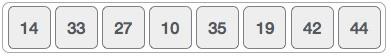
We know that merge sort first divides the whole array iteratively into equal halves unless the atomic values are achieved. We see here that an array of 8 items is divided into two arrays of size 4.

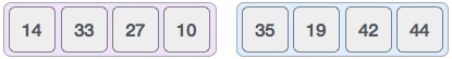
This does not change the sequence of appearance of items in the original. Now we divide these two arrays into halves.

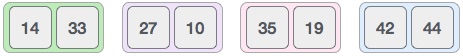
We further divide these arrays and we achieve atomic value which can no more be divided.

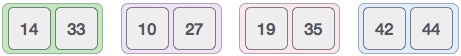
Now, we combine them in exactly the same manner as they were broken down. Please note the color codes given to these lists.

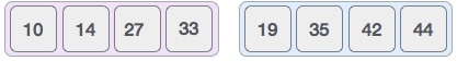
We first compare the element for each list and then combine them into another list in a sorted manner. We see that 14 and 33 are in sorted positions. We compare 27 and 10 and in the target list of 2 values we put 10 first, followed by 27. We change the order of 19 and 35 whereas 42 and 44 are placed sequentially.

In the next iteration of the combining phase, we compare lists of two data values, and merge them into a list of found data values placing all in a sorted order.

After the final merging, the list should look like this −

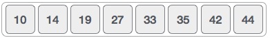
Now we should learn some programming aspects of merge sorting.

Algorithm

Merge sort keeps on dividing the list into equal halves until it can no more be divided. By definition, if it is only one element in the list, it is sorted. Then, merge sort combines the smaller sorted lists keeping the new list sorted too.

Step 1 − if it is only one element in the list it is already sorted, return.
Step 2 − divide the list recursively into two halves until it can no more be divided.
Step 3 − merge the smaller lists into new list in sorted order.

Pseudocode

We shall now see the pseudocodes for merge sort functions. As our algorithms point out two main functions − divide & merge.

Merge sort works with recursion and we shall see our implementation in the same way.

procedure mergesort( var a as array )
   if ( n == 1 ) return a

   var l1 as array = a[0] ... a[n/2]
   var l2 as array = a[n/2+1] ... a[n]

   l1 = mergesort( l1 )
   l2 = mergesort( l2 )

   return merge( l1, l2 )
end procedure

procedure merge( var a as array, var b as array )

   var c as array

   while ( a and b have elements )
      if ( a[0] > b[0] )
         add b[0] to the end of c
         remove b[0] from b
      else
         add a[0] to the end of c
         remove a[0] from a
      end if
   end while
   
   while ( a has elements )
      add a[0] to the end of c
      remove a[0] from a
   end while
   
   while ( b has elements )
      add b[0] to the end of c
      remove b[0] from b
   end while
   
   return c
 
end procedure

Merge sort is a sorting technique based on divide and conquer technique. With the worst-case time complexity being Ο(n log n), it is one of the most respected algorithms.

Implementation in C

We shall see the implementation of merge sort in C programming language here −

#include <stdio.h>
#define max 10

int a[10] = { 10, 14, 19, 26, 27, 31, 33, 35, 42, 44 };
int b[10];

void merging(int low, int mid, int high) {
   int l1, l2, i;

   for(l1 = low, l2 = mid + 1, i = low; l1 <= mid && l2 <= high; i++) {
      if(a[l1] <= a[l2])
         b[i] = a[l1++];
      else
         b[i] = a[l2++];
   }
   
   while(l1 <= mid)    
      b[i++] = a[l1++];

   while(l2 <= high)   
      b[i++] = a[l2++];

   for(i = low; i <= high; i++)
      a[i] = b[i];
}

void sort(int low, int high) {
   int mid;
   
   if(low < high) {
      mid = (low + high) / 2;
      sort(low, mid);
      sort(mid+1, high);
      merging(low, mid, high);
   } else { 
      return;
   }   
}

int main() { 
   int i;

   printf("List before sorting\n");
   
   for(i = 0; i <= max; i++)
      printf("%d ", a[i]);

   sort(0, max);

   printf("\nList after sorting\n");
   
   for(i = 0; i <= max; i++)
      printf("%d ", a[i]);
}

If we compile and run the above program, it will produce the following result −

Output

List before sorting
10 14 19 26 27 31 33 35 42 44 0
List after sorting 

0 10 14 19 26 27 31 33 35 42 44

Analysis

A recursive merge sort algorithm used to sort an array of 7 integer values. These are the steps a human would take to emulate merge sort (top-down).

In sorting n objects, merge sort has an average and worst-case performance of O(n log n). If the running time of merge sort for a list of length n is T(n), then the recurrence T(n) = 2T(n/2) + n follows from the definition of the algorithm (apply the algorithm to two lists of half the size of the original list, and add the n steps taken to merge the resulting two lists). The closed form follows from the master theorem.

In the worst case, the number of comparisons merge sort makes is equal to or slightly smaller than (n ⌈lg n⌉ - 2^⌈lg n⌉ + 1), which is between (n lg n - n + 1) and (n lg n + n + O(lg n)).

For large n and a randomly ordered input list, merge sort's expected (average) number of comparisons approaches α·n fewer than the worst case where ${\displaystyle \alpha =-1+\sum _{k=0}^{\infty }{\frac {1}{2^{k}+1}}\approx 0.2645.}$

In the worst case, merge sort does about 39% fewer comparisons than quicksort does in the average case. In terms of moves, merge sort's worst case complexity is O(n log n)—the same complexity as quicksort's best case, and merge sort's best case takes about half as many iterations as the worst case.

Merge sort is more efficient than quicksort for some types of lists if the data to be sorted can only be efficiently accessed sequentially, and is thus popular in languages such as Lisp, where sequentially accessed data structures are very common. Unlike some (efficient) implementations of quicksort, merge sort is a stable sort.

Merge sort's most common implementation does not sort in place; therefore, the memory size of the input must be allocated for the sorted output to be stored in (see below for versions that need only n/2 extra spaces).

Quick Sort

Quicksort (sometimes called partition-exchange sort) is an efficient sorting algorithm, serving as a systematic method for placing the elements of an array in order. Developed by Tony Hoare in 1959, with his work published in 1961, it is still a commonly used algorithm for sorting. When implemented well, it can be about two or three times faster than its main competitors, merge sort and heapsort.

Quicksort is a comparison sort, meaning that it can sort items of any type for which a "less-than" relation (formally, a total order) is defined. In efficient implementations it is not a stable sort, meaning that the relative order of equal sort items is not preserved. Quicksort can operate in-place on an array, requiring small additional amounts of memory to perform the sorting.

Mathematical analysis of quicksort shows that, on average, the algorithm takes O(n log n) comparisons to sort n items. In the worst case, it makes O(n²) comparisons, though this behavior is rare.

Quick sort is a highly efficient sorting algorithm and is based on partitioning of array of data into smaller arrays. A large array is partitioned into two arrays one of which holds values smaller than the specified value, say pivot, based on which the partition is made and another array holds values greater than the pivot value.

Quick sort partitions an array and then calls itself recursively twice to sort the two resulting subarrays. This algorithm is quite efficient for large-sized data sets as its average and worst case complexity are of Ο(nlogn), where n is the number of items.

Partition in Quick Sort

Following animated representation explains how to find the pivot value in an array.

The pivot value divides the list into two parts. And recursively, we find the pivot for each sub-lists until all lists contains only one element.

Quick Sort Pivot Algorithm

Based on our understanding of partitioning in quick sort, we will now try to write an algorithm for it, which is as follows.

Step 1 − Choose the highest index value has pivot
Step 2 − Take two variables to point left and right of the list excluding pivot
Step 3 − left points to the low index
Step 4 − right points to the high
Step 5 − while value at left is less than pivot move right
Step 6 − while value at right is greater than pivot move left
Step 7 − if both step 5 and step 6 does not match swap left and right
Step 8 − if left ≥ right, the point where they met is new pivot

Quick Sort Pivot Pseudocode

The pseudocode for the above algorithm can be derived as −

function partitionFunc(left, right, pivot)
   leftPointer = left -1
   rightPointer = right

   while True do
      while A[++leftPointer] < pivot do
         //do-nothing            
      end while
  
      while rightPointer > 0 && A[--rightPointer] > pivot do
         //do-nothing         
      end while
  
      if leftPointer >= rightPointer
         break
      else                
         swap leftPointer,rightPointer
      end if
  
   end while 
 
   swap leftPointer,right
   return leftPointer
 
end function

Quick Sort Algorithm

Using pivot algorithm recursively, we end up with smaller possible partitions. Each partition is then processed for quick sort. We define recursive algorithm for quicksort as follows −

Step 1 − Make the right-most index value pivot
Step 2 − partition the array using pivot value
Step 3 − quicksort left partition recursively
Step 4 − quicksort right partition recursively

Quick Sort Pseudocode

To get more into it, let see the pseudocode for quick sort algorithm −

procedure quickSort(left, right)

   if right-left <= 0
      return
   else     
      pivot = A[right]
      partition = partitionFunc(left, right, pivot)
      quickSort(left,partition-1)
      quickSort(partition+1,right)    
   end if  
   
end procedure

Quick sort is a highly efficient sorting algorithm and is based on partitioning of array of data into smaller arrays. A large array is partitioned into two arrays one of which holds values smaller than the specified value, say pivot, based on which the partition is made and another array holds values greater than the pivot value.

Implementation in C

#include <stdio.h>
#include <stdbool.h>
#define MAX 7

int intArray[MAX] = {4,6,3,2,1,9,7};

void printline(int count) {
   int i;
 
   for(i = 0;i <count-1;i++) {
      printf("=");
   }
 
   printf("=\n");
}

void display() {
   int i;
   printf("[");
 
   // navigate through all items 
   for(i = 0;i<MAX;i++) {
      printf("%d ",intArray[i]);
   }
 
   printf("]\n");
}

void swap(int num1, int num2) {
   int temp = intArray[num1];
   intArray[num1] = intArray[num2];
   intArray[num2] = temp;
}

int partition(int left, int right, int pivot) {
   int leftPointer = left -1;
   int rightPointer = right;

   while(true) {
      while(intArray[++leftPointer] < pivot) {
         //do nothing
      }
  
      while(rightPointer > 0 && intArray[--rightPointer] > pivot) {
         //do nothing
      }

      if(leftPointer >= rightPointer) {
         break;
      } else {
         printf(" item swapped :%d,%d\n", intArray[leftPointer],intArray[rightPointer]);
         swap(leftPointer,rightPointer);
      }
   }
 
   printf(" pivot swapped :%d,%d\n", intArray[leftPointer],intArray[right]);
   swap(leftPointer,right);
   printf("Updated Array: "); 
   display();
   return leftPointer;
}

void quickSort(int left, int right) {
   if(right-left <= 0) {
      return;   
   } else {
      int pivot = intArray[right];
      int partitionPoint = partition(left, right, pivot);
      quickSort(left,partitionPoint-1);
      quickSort(partitionPoint+1,right);
   }        
}

main() {
   printf("Input Array: ");
   display();
   printline(50);
   quickSort(0,MAX-1);
   printf("Output Array: ");
   display();
   printline(50);
}

If we compile and run the above program, it will produce the following result −

Output

Input Array: [4 6 3 2 1 9 7 ]
==================================================
 pivot swapped :9,7
Updated Array: [4 6 3 2 1 7 9 ]
 pivot swapped :4,1
Updated Array: [1 6 3 2 4 7 9 ]
 item swapped :6,2
 pivot swapped :6,4
Updated Array: [1 2 3 4 6 7 9 ]
 pivot swapped :3,3
Updated Array: [1 2 3 4 6 7 9 ]
Output Array: [1 2 3 4 6 7 9 ] 

==================================================

Worst-case analysis

The most unbalanced partition occurs when the pivot divides the list into two sublists of sizes 0 and n − 1. This may occur if the pivot happens to be the smallest or largest element in the list, or in some implementations (e.g., the Lomuto partition scheme as described above) when all the elements are equal.

If this happens repeatedly in every partition, then each recursive call processes a list of size one less than the previous list. Consequently, we can make n − 1 nested calls before we reach a list of size 1. This means that the call tree is a linear chain of n − 1 nested calls. The ith call does O(n − i) work to do the partition, and ${\displaystyle \textstyle \sum _{i=0}^{n}(n-i)=O(n^{2})}$, so in that case Quicksort takes O(n²) time.

Best-case analysis

In the most balanced case, each time we perform a partition we divide the list into two nearly equal pieces. This means each recursive call processes a list of half the size. Consequently, we can make only log₂ n nested calls before we reach a list of size 1. This means that the depth of the call tree is log₂ n. But no two calls at the same level of the call tree process the same part of the original list; thus, each level of calls needs only O(n) time all together (each call has some constant overhead, but since there are only O(n) calls at each level, this is subsumed in the O(n) factor). The result is that the algorithm uses only O(n log n) time.

Average-case analysis

To sort an array of n distinct elements, quicksort takes O(n log n) time in expectation, averaged over all n! permutations of n elements with equal probability. We list here three common proofs to this claim providing different insights into quicksort's workings.

Space complexity

The space used by quicksort depends on the version used.

The in-place version of quicksort has a space complexity of O(log n), even in the worst case, when it is carefully implemented using the following strategies:

• in-place partitioning is used. This unstable partition requires O(1) space.
• After partitioning, the partition with the fewest elements is (recursively) sorted first, requiring at most O(log n) space. Then the other partition is sorted using tail recursion or iteration, which doesn't add to the call stack. This idea, as discussed above, was described by R. Sedgewick, and keeps the stack depth bounded by O(log n).

Quicksort with in-place and unstable partitioning uses only constant additional space before making any recursive call. Quicksort must store a constant amount of information for each nested recursive call. Since the best case makes at most O(log n) nested recursive calls, it uses O(log n) space. However, without Sedgewick's trick to limit the recursive calls, in the worst case quicksort could make O(n) nested recursive calls and need O(n) auxiliary space.

From a bit complexity viewpoint, variables such as lo and hi do not use constant space; it takes O(log n) bits to index into a list of n items. Because there are such variables in every stack frame, quicksort using Sedgewick's trick requires O((log n)²) bits of space. This space requirement isn't too terrible, though, since if the list contained distinct elements, it would need at least O(n log n) bits of space.

Another, less common, not-in-place, version of quicksort uses O(n) space for working storage and can implement a stable sort. The working storage allows the input array to be easily partitioned in a stable manner and then copied back to the input array for successive recursive calls. Sedgewick's optimization is still appropriate.

Quick Sort

The basic version of quick sort algorithm was invented by C. A. R. Hoare in 1960 and formally introduced quick sort in 1962.  It is used on the principle of divide-and-conquer. Quick sort is an algorithm of choice in many situations because it is not difficult to implement, it is a good "general purpose" sort and it consumes relatively fewer resources during execution.

 

Good points

• It is in-place since it uses only a small auxiliary stack.
• It requires only n log(n) time to sort n items.
• It has an extremely short inner loop
• This algorithm has been subjected to a thorough mathematical analysis, a very precise statement can be made about performance issues.

Bad Points

• It is recursive. Especially if recursion is not available, the implementation is extremely complicated.
• It requires quadratic (i.e., n²) time in the worst-case.
• It is fragile i.e., a simple mistake in the implementation can go unnoticed and cause it to perform badly.

Quick sort works by partitioning a given array A[p . . r] into two non-empty sub array A[p . . q] and A[q+1 . . r] such that every key in A[p . . q] is less than or equal to every key in A[q+1 . . r]. Then the two subarrays are sorted by recursive calls to Quick sort. The exact position of the partition depends on the given array and index q is computed as a part of the partitioning procedure.

QuickSort

1. If p < r then
2.     q Partition (A, p, r)
3.     Recursive call to Quick Sort (A, p, q)
4.     Recursive call to Quick Sort (A, q + r, r)

Note that to sort entire array, the initial call Quick Sort (A, 1, length[A])

As a first step, Quick Sort chooses as pivot one of the items in the array to be sorted. Then array is then partitioned on either side of the pivot. Elements that are less than or equal to pivot will move toward the left and elements that are greater than or equal to pivot will move toward the right.

 

Partitioning the Array

Partitioning procedure rearranges the subarrays in-place.

PARTITION (A, p, r)

1. x ← A[p]
2. i ← p-1
3. j ← r+1
4. while TRUE do
5.     Repeat j ← j-1
6.     until A[j] ≤ x
7.     Repeat i ← i+1
8.     until A[i] ≥ x
9.     if i < j
10.         then exchange A[i] ↔ A[j]
11.         else return j

Partition selects the first key, A[p] as a pivot key about which the array will partitioned:

Keys ≤  A[p] will be moved towards the left .
Keys ≥ A[p] will be moved towards the right.

The running time of the partition procedure is (n) where n = r - p +1 which is the number of keys in the array.
Another argument that running  time of PARTITION on a subarray of size (n) is as follows: Pointer i and pointer j start at each end and move towards each other, conveying somewhere in the middle. The total number of times that i can be incremented and j can be decremented is therefore O(n). Associated with each increment or decrement there are O(1) comparisons and swaps. Hence, the total time is O(n).

 

Array of Same Elements

Since all the elements are equal, the "less than or equal" teat in lines 6 and 8 in the PARTITION (A, p, r) will always be true. this simply means that repeat loop all stop at once. Intuitively, the first repeat loop moves j to the left; the second repeat loop moves i to the right. In this case, when all elements are equal, each repeat loop moves i and j towards the middle one space. They meet in the middle, so q= Floor(p+r/2). Therefore, when all elements in the array A[p . . r] have the same value equal to Floor(p+r/2).

 

Performance of Quick Sort

The running time of quick sort depends on whether partition is balanced or unbalanced, which in turn depends on which elements of an array to be sorted are used for partitioning.
A very good partition splits an array up into two equal sized arrays. A bad partition, on other hand, splits an array up into two arrays of very different sizes. The worst partition puts only one element in one array and all other elements in the other array. If the partitioning is balanced, the Quick sort runs asymptotically as fast as merge sort. On the other hand, if partitioning is unbalanced, the Quick sort runs asymptotically as slow as insertion sort.

Best Case

The best thing that could happen in Quick sort would be that each partitioning stage divides the array exactly in half. In other words, the best to be a median of the keys in A[p . . r] every time procedure 'Partition' is called. The procedure 'Partition' always split the array to be sorted into two equal sized arrays.
If the procedure 'Partition' produces two regions of size n/2. the recurrence relation is then

T(n) = T(n/2) + T(n/2) + (n)
       = 2T(n/2) + (n)

And from case 2 of Master theorem

        T(n) = (n lg n)

 

Worst case Partitioning

The worst-case occurs if given array A[1 . . n] is already sorted. The PARTITION (A, p, r) call always return p so successive calls to partition will split arrays of length n, n-1, n-2, . . . , 2 and running time proportional to n + (n-1) + (n-2) + . . . + 2 = [(n+2)(n-1)]/2 = (n²). The worst-case also occurs if A[1 . . n] starts out in reverse order.

 

 

Randomized Quick Sort

In the randomized version of Quick sort we impose a distribution on input. This does not improve the worst-case running time independent of the input ordering.
In this version we choose a random key for the pivot. Assume that procedure Random (a, b) returns a random integer in the range [a, b); there are b-a+1 integers in the range and procedure is equally likely to return one of them. The new partition procedure, simply implemented the swap before actually partitioning.

RANDOMIZED_PARTITION (A, p, r)

i ← RANDOM (p, r)
Exchange A[p] ↔ A[i]
return PARTITION (A, p, r)

Now randomized quick sort call the above procedure in place of PARTITION

RANDOMIZED_QUICKSORT (A, p, r)

If p < r then
    q ← RANDOMIZED_PARTITION (A, p, r)
    RANDOMIZED_QUICKSORT (A, p, q)
    RANDOMIZED_QUICKSORT (A, q+1, r)

Like other randomized algorithms, RANDOMIZED_QUICKSORT has the property that no particular input elicits its worst-case behavior; the behavior of algorithm only depends on the random-number generator. Even intentionally, we cannot produce a bad input for RANDOMIZED_QUICKSORT unless we can predict generator will produce next.

 

Analysis of Quick sort

Worst-case

Let T(n) be the worst-case time for QUICK SORT on input size n. We have a recurrence

T(n) = max_1≤q≤n-1 (T(q) + T(n-q)) + (n)             --------- 1

where q runs from 1 to n-1, since the partition produces two regions, each having size at least 1.
Now we guess that T(n) ≤ cn² for some constant c.
Substituting our guess in equation 1.We get

    T(n) = max_1≤q≤n-1 (cq² ) + c(n - q²)) + (n)
           = c max (q² + (n - q)²) +  (n)

Since the second derivative of expression q² + (n-q)²  with respect to q is positive. Therefore, expression achieves a maximum over the range 1≤ q  ≤ n -1 at one of the endpoints. This gives the bound max (q² + (n - q)²)) 1 + (n -1)^{2 =} n² + 2(n -1).
Continuing with our bounding of T(n) we get

    T(n) ≤ c [n² - 2(n-1)] + (n)
            = cn² - 2c(n-1) + (n)

Since we can pick the constant so that the 2c(n -1) term dominates the (n) term we have

     T(n)  ≤  cn²

Thus the worst-case running time of quick sort is (n²).

 

Average-case Analysis

If the split induced by RANDOMIZED_PARTITION puts constant fraction of elements on one side of the partition, then the recurrence tree has depth (lgn) and (n) work is performed at (lg n) of these level. This is an intuitive argument why the average-case running time of  RANDOMIZED_QUICKSORT is (n lg n).
Let T(n) denotes the average time required to sort an array of n elements. A call to RANDOMIZED_QUICKSORT with a 1 element array takes a constant time, so we have T(1) =  (1).
After the split RANDOMIZED_QUICKSORT calls itself to sort two subarrays. The average time to sort an array A[1 . . q] is T[q] and the average time to sort an array A[q+1 . . n] is T[n-q]. We have

        T(n) = 1/n (T(1) + T(n-1) + ^n-1∑_q=1 T(q) + T(n-q))) + (n)    ----- 1

We know from worst-case analysis

T(1) =  (1) and T(n -1) = O(n²)
T(n) = 1/n ((1) + O(n²)) + 1/n ^n-1∑_q=1 (r(q) + T(n - q)) ₊ (n)
       = 1/n  ^n-1∑_q=1(T(q) + T(n - q)) + (n)                          ------- 2
       = 1/n[2  ^n-1∑_k=1(T(k)] + (n)
       = 2/n ^n-1∑_k=1(T(k) + (n)                                           --------- 3

Solve the above recurrence using substitution method. Assume inductively that T(n) ≤ anlgn + b for some constants a > 0 and b > 0.
If we can pick 'a' and 'b' large enough so that n lg n + b > T(1). Then for n > 1, we have

T(n) ≥ ^n-1∑_k=1 2/n (aklgk + b) + (n)
        = 2a/n ^n-1∑_k=1 klgk - 1/8(n²) +  2b/n (n -1) + (n)     ------- 4

At this point we are claiming that

^n-1∑_k=1 klgk  ≤  1/2 n² lgn - 1/8(n²)

Stick this claim in the equation 4 above and we get

T(n)  ≤   2a/n [1/2 n²  lgn - 1/8(n²)] + 2/n b(n -1) + (n)
         ≤  anlgn - an/4 + 2b + (n)                                  ---------- 5

In the above equation, we see that (n) + b and an/4 are polynomials and we certainly can choose 'a' large enough so that an/4 dominates (n)  + b.
We conclude that QUICKSORT's average running time is (n lg(n)).

Conclusion
Quick sort is an in place sorting algorithm whose worst-case running time is (n²) and expected running time is (n lg n) where constants hidden in (n lg n) are small.

 

 

Implementation

void quickSort(int numbers[], int array_size)
{
  q_sort(numbers, 0, array_size - 1);
}


void q_sort(int numbers[], int left, int right)
{
  int pivot, l_hold, r_hold;

  l_hold = left;
  r_hold = right;
  pivot = numbers[left];
  while (left < right)
  {
    while ((numbers[right] >= pivot) && (left < right))
      right--;
    if (left != right)
    {
      numbers[left] = numbers[right];
      left++;
    }
    while ((numbers[left] <= pivot) && (left < right))
      left++;
    if (left != right)
    {
      numbers[right] = numbers[left];
      right--;
    }
  }
  numbers[left] = pivot;
  pivot = left;
  left = l_hold;
  right = r_hold;
  if (left < pivot)
    q_sort(numbers, left, pivot-1);
  if (right > pivot)
    q_sort(numbers, pivot+1, right);
}

Strassen’s Matrix Multiplication

In linear algebra, the Strassen algorithm, named after Volker Strassen, is an algorithm for matrix multiplication. It is faster than the standard matrix multiplication algorithm and is useful in practice for large matrices, but would be slower than the fastest known algorithms for extremely large matrices.

Strassen's algorithm works for any ring, such as plus/multiply, but not all semirings, such as min/plus or boolean algebra, where the naive algorithm still works, and so called combinatorial matrix multiplication.

Given two square matrices A and B of size n x n each, find their multiplication matrix.

Naive Method
Following is a simple way to multiply two matrices.

void multiply(int A[][N], int B[][N], int C[][N]) {     for (int i = 0; i < N; i++)     {         for (int j = 0; j < N; j++)         {             C[i][j] = 0;             for (int k = 0; k < N; k++)             {                 C[i][j] += A[i][k]*B[k][j];             }         }     } }

Time Complexity of above method is O(N3).

Divide and Conquer 
Following is simple Divide and Conquer method to multiply two square matrices.
1) Divide matrices A and B in 4 sub-matrices of size N/2 x N/2 as shown in the below diagram.
2) Calculate following values recursively. ae + bg, af + bh, ce + dg and cf + dh.

In the above method, we do 8 multiplications for matrices of size N/2 x N/2 and 4 additions. Addition of two matrices takes O(N2) time. So the time complexity can be written as

T(N) = 8T(N/2) + O(N2)  

From Master's Theorem, time complexity of above method is O(N3)
which is unfortunately same as the above naive method.

Simple Divide and Conquer also leads to O(N3), can there be a better way?
In the above divide and conquer method, the main component for high time complexity is 8 recursive calls. The idea of Strassen’s method is to reduce the number of recursive calls to 7. Strassen’s method is similar to above simple divide and conquer method in the sense that this method also divide matrices to sub-matrices of size N/2 x N/2 as shown in the above diagram, but in Strassen’s method, the four sub-matrices of result are calculated using following formulae.

Time Complexity of Strassen’s Method
Addition and Subtraction of two matrices takes O(N2) time. So time complexity can be written as

T(N) = 7T(N/2) +  O(N2)

From Master's Theorem, time complexity of above method is 
O(NLog7) which is approximately O(N2.8074)

Generally Strassen’s Method is not preferred for practical applications for following reasons.
1) The constants used in Strassen’s method are high and for a typical application Naive method works better.
2) For Sparse matrices, there are better methods especially designed for them.
3) The submatrices in recursion take extra space.
4) Because of the limited precision of computer arithmetic on noninteger values, larger errors accumulate in Strassen’s algorithm than in Naive Method

Asymptotic complexity

The standard matrix multiplication takes approximately 2N³ (where N = 2ⁿ) arithmetic operations (additions and multiplications); the asymptotic complexity is Θ(N³).

The number of additions and multiplications required in the Strassen algorithm can be calculated as follows: let f(n) be the number of operations for a 2ⁿ × 2ⁿ matrix. Then by recursive application of the Strassen algorithm, we see that f(n) = 7f(n−1) + ℓ4ⁿ, for some constant ℓ that depends on the number of additions performed at each application of the algorithm. Hence f(n) = (7 + o(1))ⁿ, i.e., the asymptotic complexity for multiplying matrices of size N = 2ⁿ using the Strassen algorithm is

${\displaystyle O([7+o(1)]^{n})=O(N^{\log _{2}7+o(1)})\approx O(N^{2.8074})}$.

The reduction in the number of arithmetic operations however comes at the price of a somewhat reduced numerical stability, and the algorithm also requires significantly more memory compared to the naive algorithm. Both initial matrices must have their dimensions expanded to the next power of 2, which results in storing up to four times as many elements, and the seven auxiliary matrices each contain a quarter of the elements in the expanded ones.

The description above states that the matrices are square, and the size is a power of two, and that padding should be used if needed. This restriction allows the matrices to be split in half, recursively, until limit of scalar multiplication is reached. The restriction simplifies the explanation, and analysis of complexity, but is not actually necessary; and in fact, padding the matrix as described will increase the computation time and can easily eliminate the fairly narrow time savings obtained by using the method in the first place.

A good implementation will observe the following:

• It is not necessary or desirable to use the Strassen algorithm down to the limit of scalars. Compared to conventional matrix multiplication, the algorithm adds a considerable ${\displaystyle O(n^{2})}$ workload in addition/subtractions; so below a certain size, it will be better to use conventional multiplication. Thus, for instance, if you start with matrices that are 1600x1600, there is no need to pad to 2048x2048, since you could subdivide down to 25x25 and then use conventional multiplication at that level.
• The method can indeed be applied to square matrices of any dimension. If the dimension is even, they are split in half as described. If the dimension is odd, zero padding by one row and one column is applied first. Such padding can be applied on-the-fly and lazily, and the extra rows and columns discarded as the result is formed. For instance, suppose the matrices are 199x199. They can be split so that the upper-left portion is 100x100 and the lower-right is 99x99. Wherever the operations require it, dimensions of 99 are zero padded to 100 first. Note, for instance, that the product ${\displaystyle M_{2}}$ is only used in the lower row of the output, so is only required to be 99 rows high; and thus the left factor ${\displaystyle (A_{2,1}+A_{2,2})}$ used to generate it need only be 99 rows high; accordingly, there is no need to pad that sum to 100 rows; it is only necessary to pad ${\displaystyle A_{2,2}}$ to 100 columns to match ${\displaystyle A_{2,1}}$.

Furthermore, there is no need for the matrices to be square. Non-square matrices can be split in half using the same methods, yielding smaller non-square matrices. If the matrices are sufficiently non-square it will be worthwhile reducing the initial operation to more square products, using simple methods which are essentially ${\displaystyle O(n^{2})}$, for instance:

• A product of size [2N x N] * [N x 10N] can be done as 20 separate [N x N] * [N x N] operations, arranged to form the result;
• A product of size [N x 10N] * [10N x N] can be done as 10 separate [N x N] * [N x N] operations, summed to form the result.

These techniques will make the implementation more complicated, compared to simply padding to a power-of-two square; however, it is a reasonable assumption that anyone undertaking an implementation of Strassen, rather than conventional, multiplication, will place a higher priority on computational efficiency than on simplicity of the implementation.

[https://en.wikipedia.org/wiki/Divide_and_conquer_algorithm]

[https://www.tutorialspoint.com/data_structures_algorithms/binary_search_program_in_c.htm]

[https://www.tutorialspoint.com/data_structures_algorithms/divide_and_conquer.htm]

[https://www.tutorialspoint.com/data_structures_algorithms/quick_sort_algorithm.htm]

[https://www.tutorialspoint.com/data_structures_algorithms/merge_sort_algorithm.htm]

[https://en.wikipedia.org/wiki/Quicksort]

[http://www.personal.kent.edu/~rmuhamma/Algorithms/MyAlgorithms/Sorting/quickSort.htm]

[https://en.wikipedia.org/wiki/Strassen_algorithm]

[http://www.geeksforgeeks.org/strassens-matrix-multiplication/]